数据结构

什么是数据结构？

在计算机科学领域，数据结构是一种数据组织、管理和存储格式，通常被选择用来高效访问数据

In computer science, a data structure is a data organization, management, and storage format that is usually chosen for efficient access to data

数据结构是一种存储和组织数据的方式，旨在便于访问和修改

A data structure is a way to store and organize data in order to facilitate access and modifications

数组

在计算机科学中，数组是由一组元素（值或变量）组成的数据结构，每个元素有至少一个索引或键来标识

In computer science, an array is a data structure consisting of a collection of elements (values or variables), each identified by at least one array index or key

概述

因为数组内的元素是连续存储的，所以数组中元素的地址，可以通过其索引计算出来，例如：

int[] array = {1,2,3,4,5}

知道了数组的数据起始地址 $BaseAddress$，就可以由公式 $BaseAddress+i\ast size$ 计算出索引 $i$ 元素的地址

• $i$ 即索引，在 Java、C 等语言都是从 0 开始
• $size$ 是每个元素占用字节，例如 $int$ 占 $4$，$double$ 占 $8$

小测试

byte[] array = {1,2,3,4,5}

已知 array 的数据的起始地址是 0x7138f94c8，那么元素 3 的地址是什么？

答：0x7138f94c8 + 2 * 1 = 0x7138f94ca

空间占用

Java 中数组结构为

• 8 字节 markword
• 4 字节 class 指针（压缩 class 指针的情况）
• 4 字节 数组大小（决定了数组最大容量是 $2^{32}$）
• 数组元素 + 对齐字节（java 中所有对象大小都是 8 字节的整数倍[^12]，不足的要用对齐字节补足）

例如

int[] array = {1, 2, 3, 4, 5};

的大小为 40 个字节，组成如下

8 + 4 + 4 + 5*4 + 4(alignment)

随机访问性能

即根据索引查找元素，时间复杂度是 $O(1)$

动态数组

java 版本

public class DynamicArray implements Iterable<Integer> {
    private int size = 0; // 逻辑大小
    private int capacity = 8; // 容量
    private int[] array = {};


    /**
     * 向最后位置 [size] 添加元素
     *
     * @param element 待添加元素
     */
    public void addLast(int element) {
        add(size, element);
    }

    /**
     * 向 [0 .. size] 位置添加元素
     *
     * @param index   索引位置
     * @param element 待添加元素
     */
    public void add(int index, int element) {
        checkAndGrow();

        // 添加逻辑
        if (index >= 0 && index < size) {
            // 向后挪动, 空出待插入位置
            System.arraycopy(array, index,
                    array, index + 1, size - index);
        }
        array[index] = element;
        size++;
    }

    private void checkAndGrow() {
        // 容量检查
        if (size == 0) {
            array = new int[capacity];
        } else if (size == capacity) {
            // 进行扩容, 1.5 1.618 2
            capacity += capacity >> 1;
            int[] newArray = new int[capacity];
            System.arraycopy(array, 0,
                    newArray, 0, size);
            array = newArray;
        }
    }

    /**
     * 从 [0 .. size) 范围删除元素
     *
     * @param index 索引位置
     * @return 被删除元素
     */
    public int remove(int index) { // [0..size)
        int removed = array[index];
        if (index < size - 1) {
            // 向前挪动
            System.arraycopy(array, index + 1,
                    array, index, size - index - 1);
        }
        size--;
        return removed;
    }


    /**
     * 查询元素
     *
     * @param index 索引位置, 在 [0..size) 区间内
     * @return 该索引位置的元素
     */
    public int get(int index) {
        return array[index];
    }

    /**
     * 遍历方法1
     *
     * @param consumer 遍历要执行的操作, 入参: 每个元素
     */
    public void foreach(Consumer<Integer> consumer) {
        for (int i = 0; i < size; i++) {
            // 提供 array[i]
            // 返回 void
            consumer.accept(array[i]);
        }
    }

    /**
     * 遍历方法2 - 迭代器遍历
     */
    @Override
    public Iterator<Integer> iterator() {
        return new Iterator<Integer>() {
            int i = 0;

            @Override
            public boolean hasNext() { // 有没有下一个元素
                return i < size;
            }

            @Override
            public Integer next() { // 返回当前元素,并移动到下一个元素
                return array[i++];
            }
        };
    }

    /**
     * 遍历方法3 - stream 遍历
     *
     * @return stream 流
     */
    public IntStream stream() {
        return IntStream.of(Arrays.copyOfRange(array, 0, size));
    }
}

• 这些方法实现，都简化了 index 的有效性判断，假设输入的 index 都是合法的

插入或删除性能

头部位置，时间复杂度是 $O(n)$

中间位置，时间复杂度是 $O(n)$

尾部位置，时间复杂度是 $O(1)$（均摊来说）

二维数组

int[][] array = {
    {11, 12, 13, 14, 15},
    {21, 22, 23, 24, 25},
    {31, 32, 33, 34, 35},
};

内存图如下

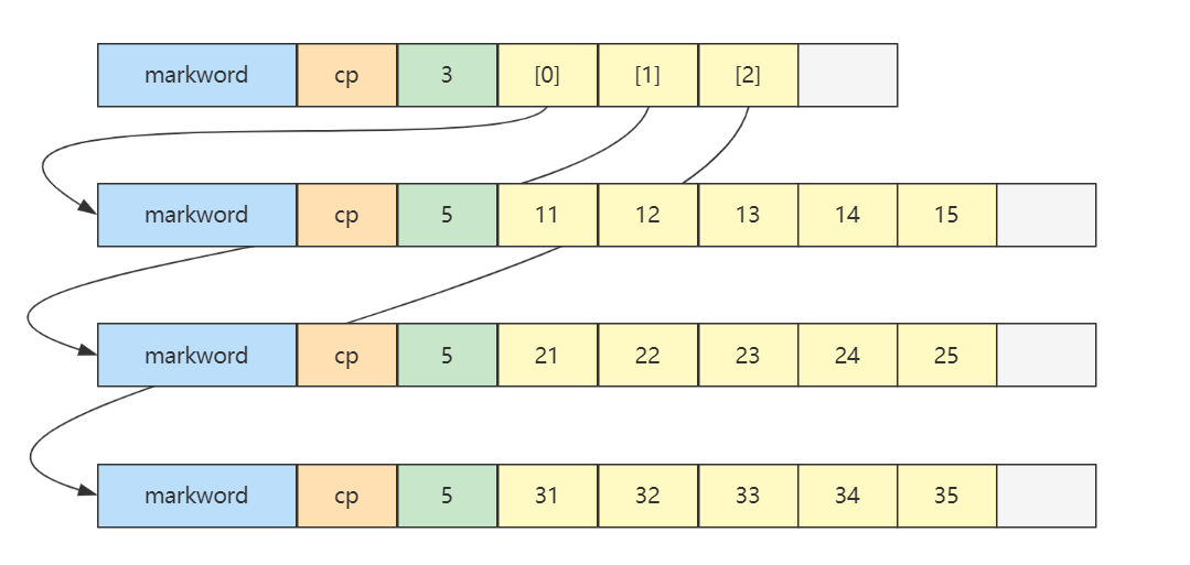
• 二维数组占 32 个字节，其中 array[0]，array[1]，array[2] 三个元素分别保存了指向三个一维数组的引用

• 三个一维数组各占 40 个字节

• 它们在内层布局上是连续的

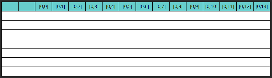
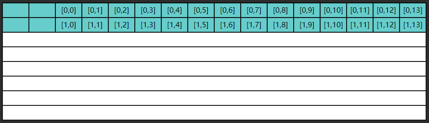
更一般的，对一个二维数组 $Array[m][n]$

• $m$ 是外层数组的长度，可以看作 row 行
• $n$ 是内层数组的长度，可以看作 column 列
• 当访问 $Array[i][j]$，$0\le i<m,0\le j<n$时，就相当于
  • 先找到第 $i$ 个内层数组（行）
  • 再找到此内层数组中第 $j$ 个元素（列）

小测试

Java 环境下（不考虑类指针和引用压缩，此为默认情况），有下面的二维数组

byte[][] array = {
    {11, 12, 13, 14, 15},
    {21, 22, 23, 24, 25},
    {31, 32, 33, 34, 35},
};

已知 array 对象起始地址是 0x1000，那么 23 这个元素的地址是什么？

答：

• 起始地址 0x1000
• 外层数组大小：16字节对象头 + 3元素 * 每个引用4字节 + 4 对齐字节 = 32 = 0x20
• 第一个内层数组大小：16字节对象头 + 5元素 * 每个byte1字节 + 3 对齐字节 = 24 = 0x18
• 第二个内层数组，16字节对象头 = 0x10，待查找元素索引为 2
• 最后结果 = 0x1000 + 0x20 + 0x18 + 0x10 + 2*1 = 0x104a

局部性原理

这里只讨论空间局部性

• cpu 读取内存（速度慢）数据后，会将其放入高速缓存（速度快）当中，如果后来的计算再用到此数据，在缓存中能读到的话，就不必读内存了
• 缓存的最小存储单位是缓存行（cache line），一般是 64 bytes，一次读的数据少了不划算啊，因此最少读 64 bytes 填满一个缓存行，因此读入某个数据时也会读取其临近的数据，这就是所谓空间局部性

对效率的影响

比较下面 ij 和 ji 两个方法的执行效率

int rows = 1000000;
int columns = 14;
int[][] a = new int[rows][columns];

StopWatch sw = new StopWatch();
sw.start("ij");
ij(a, rows, columns);
sw.stop();
sw.start("ji");
ji(a, rows, columns);
sw.stop();
System.out.println(sw.prettyPrint());

ij 方法

public static void ij(int[][] a, int rows, int columns) {
    long sum = 0L;
    for (int i = 0; i < rows; i++) {
        for (int j = 0; j < columns; j++) {
            sum += a[i][j];
        }
    }
    System.out.println(sum);
}

ji 方法

public static void ji(int[][] a, int rows, int columns) {
    long sum = 0L;
    for (int j = 0; j < columns; j++) {
        for (int i = 0; i < rows; i++) {
            sum += a[i][j];
        }
    }
    System.out.println(sum);
}

执行结果

0
0
StopWatch '': running time = 96283300 ns
---------------------------------------------
ns         %     Task name
---------------------------------------------
016196200  017%  ij
080087100  083%  ji

可以看到 ij 的效率比 ji 快很多，为什么呢？

• 缓存是有限的，当新数据来了后，一些旧的缓存行数据就会被覆盖
• 如果不能充分利用缓存的数据，就会造成效率低下

以 ji 执行为例，第一次内循环要读入 $[0,0]$ 这条数据，由于局部性原理，读入 $[0,0]$ 的同时也读入了 $[0,1]...[0,13]$，如图所示

但很遗憾，第二次内循环要的是 $[1,0]$ 这条数据，缓存中没有，于是再读入了下图的数据

这显然是一种浪费，因为 $[0,1]...[0,13]$ 包括 $[1,1]...[1,13]$ 这些数据虽然读入了缓存，却没有及时用上，而缓存的大小是有限的，等执行到第九次内循环时

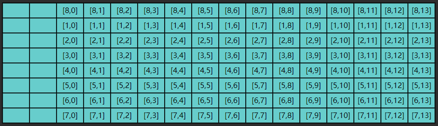
缓存的第一行数据已经被新的数据 $[8,0]...[8,13]$ 覆盖掉了，以后如果再想读，比如 $[0,1]$，又得到内存去读了

同理可以分析 ij 函数则能充分利用局部性原理加载到的缓存数据

举一反三

1. I/O 读写时同样可以体现局部性原理

2. 数组可以充分利用局部性原理，那么链表呢？

   答：链表不行，因为链表的元素并非相邻存储

越界检查

java 中对数组元素的读写都有越界检查，类似于下面的代码

bool is_within_bounds(int index) const        
{ 
    return 0 <= index && index < length(); 
}

• 代码位置：openjdk\src\hotspot\share\oops\arrayOop.hpp

只不过此检查代码，不需要由程序员自己来调用，JVM 会帮我们调用

链表

在计算、机科学中，链表是数据元素的线性集合，其每个元素都指向下一个元素，元素存储上并不连续

In computer science, a linked list is a linear collection of data elements whose order is not given by their physical placement in memory. Instead, each element points to the next.

概述

• 单向链表，每个元素只知道其下一个元素是谁

• 双向链表，每个元素知道其上一个元素和下一个元素

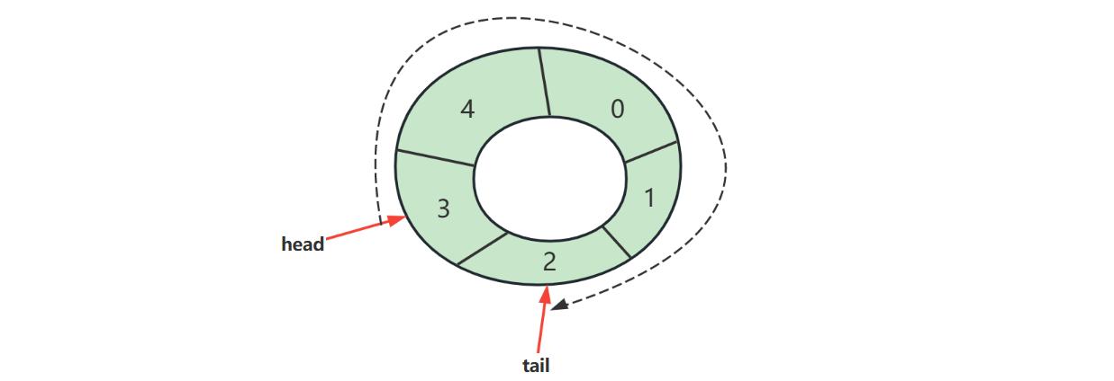
• 循环链表，通常的链表尾节点 tail 指向的都是 null，而循环链表的 tail 指向的是头节点 head

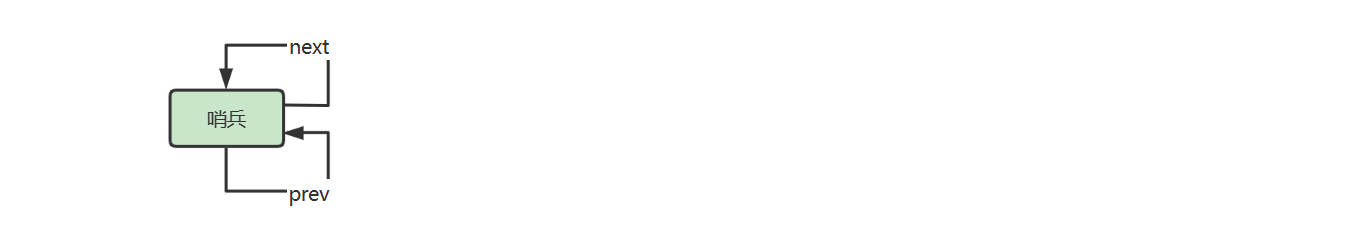
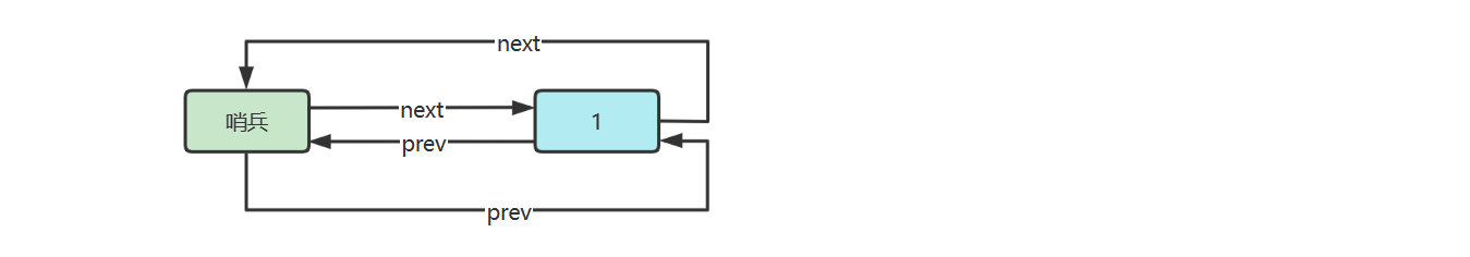
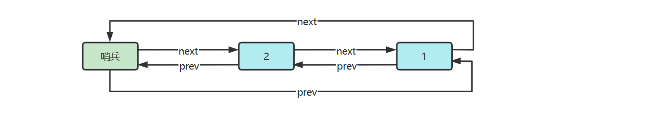
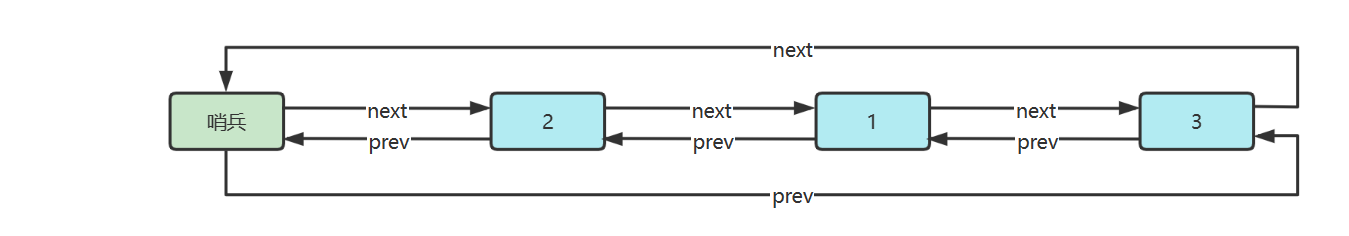
链表内还有一种特殊的节点称为哨兵（Sentinel）节点，也叫做哑元（ Dummy）节点，它不存储数据，通常用作头尾，用来简化边界判断，如下图所示

随机访问性能

根据 index 查找，时间复杂度 $O(n)$

插入或删除性能

• 起始位置：$O(1)$
• 结束位置：如果已知 tail 尾节点是 $O(1)$，不知道 tail 尾节点是 $O(n)$
• 中间位置：根据 index 查找时间 + $O(1)$

单向链表

根据单向链表的定义，首先定义一个存储 value 和 next 指针的类 Node，和一个描述头部节点的引用

public class SinglyLinkedList {
    
    private Node head; // 头部节点
    
    private static class Node { // 节点类
        int value;
        Node next;

        public Node(int value, Node next) {
            this.value = value;
            this.next = next;
        }
    }
}

• Node 定义为内部类，是为了对外隐藏实现细节，没必要让类的使用者关心 Node 结构
• 定义为 static 内部类，是因为 Node 不需要与 SinglyLinkedList 实例相关，多个 SinglyLinkedList实例能共用 Node 类定义

头部添加

public class SinglyLinkedList {
    // ...
    public void addFirst(int value) {
		this.head = new Node(value, this.head);
    }
}

• 如果 this.head == null，新增节点指向 null，并作为新的 this.head
• 如果 this.head != null，新增节点指向原来的 this.head，并作为新的 this.head
  • 注意赋值操作执行顺序是从右到左

while 遍历

public class SinglyLinkedList {
    // ...
    public void loop() {
        Node curr = this.head;
        while (curr != null) {
            // 做一些事
            curr = curr.next;
        }
    }
}

for 遍历

public class SinglyLinkedList {
    // ...
    public void loop() {
        for (Node curr = this.head; curr != null; curr = curr.next) {
            // 做一些事
        }
    }
}

• 以上两种遍历都可以把要做的事以 Consumer 函数的方式传递进来
  • Consumer 的规则是一个参数，无返回值，因此像 System.out::println 方法等都是 Consumer
  • 调用 Consumer 时，将当前节点 curr.value 作为参数传递给它

迭代器遍历

public class SinglyLinkedList implements Iterable<Integer> {
    // ...
    private class NodeIterator implements Iterator<Integer> {
        Node curr = head;
        
        public boolean hasNext() {
            return curr != null;
        }

        public Integer next() {
            int value = curr.value;
            curr = curr.next;
            return value;
        }
    }
    
    public Iterator<Integer> iterator() {
        return new NodeIterator();
    }
}

• hasNext 用来判断是否还有必要调用 next
• next 做两件事
  • 返回当前节点的 value
  • 指向下一个节点
• NodeIterator 要定义为非 static 内部类，是因为它与 SinglyLinkedList 实例相关，是对某个 SinglyLinkedList 实例的迭代

递归遍历

public class SinglyLinkedList implements Iterable<Integer> {
    // ...
    public void loop() {
        recursion(this.head);
    }

    private void recursion(Node curr) {
        if (curr == null) {
            return;
        }
        // 前面做些事
        recursion(curr.next);
        // 后面做些事
    }
}

尾部添加

public class SinglyLinkedList {
    // ...
    private Node findLast() {
        if (this.head == null) {
            return null;
        }
        Node curr;
        for (curr = this.head; curr.next != null; ) {
            curr = curr.next;
        }
        return curr;
    }
    
    public void addLast(int value) {
        Node last = findLast();
        if (last == null) {
            addFirst(value);
            return;
        }
        last.next = new Node(value, null);
    }
}

• 注意，找最后一个节点，终止条件是 curr.next == null
• 分成两个方法是为了代码清晰，而且 findLast() 之后还能复用

尾部添加多个

public class SinglyLinkedList {
    // ...
	public void addLast(int first, int... rest) {
        
        Node sublist = new Node(first, null);
        Node curr = sublist;
        for (int value : rest) {
            curr.next = new Node(value, null);
            curr = curr.next;
        }
        
        Node last = findLast();
        if (last == null) {
            this.head = sublist;
            return;
        }
        last.next = sublist;
    }
}

• 先串成一串 sublist
• 再作为一个整体添加

根据索引获取

public class SinglyLinkedList {
    // ...
	private Node findNode(int index) {
        int i = 0;
        for (Node curr = this.head; curr != null; curr = curr.next, i++) {
            if (index == i) {
                return curr;
            }
        }
        return null;
    }
    
    private IllegalArgumentException illegalIndex(int index) {
        return new IllegalArgumentException(String.format("index [%d] 不合法%n", index));
    }
    
    public int get(int index) {
        Node node = findNode(index);
        if (node != null) {
            return node.value;
        }
        throw illegalIndex(index);
    }
}

• 同样，分方法可以实现复用

插入

public class SinglyLinkedList {
    // ...
	public void insert(int index, int value) {
        if (index == 0) {
            addFirst(value);
            return;
        }
        Node prev = findNode(index - 1); // 找到上一个节点
        if (prev == null) { // 找不到
            throw illegalIndex(index);
        }
        prev.next = new Node(value, prev.next);
    }
}

• 插入包括下面的删除，都必须找到上一个节点

删除

public class SinglyLinkedList {
    // ...
	public void remove(int index) {
        if (index == 0) {
            if (this.head != null) {
                this.head = this.head.next;
                return;
            } else {
                throw illegalIndex(index);
            }
        }
        Node prev = findNode(index - 1);
        Node curr;
        if (prev != null && (curr = prev.next) != null) {
            prev.next = curr.next;
        } else {
            throw illegalIndex(index);
        }
    }
}

• 第一个 if 块对应着 removeFirst 情况
• 最后一个 if 块对应着至少得两个节点的情况
  • 不仅仅判断上一个节点非空，还要保证当前节点非空

单向链表（带哨兵）

观察之前单向链表的实现，发现每个方法内几乎都有判断是不是 head 这样的代码，能不能简化呢？

用一个不参与数据存储的特殊 Node 作为哨兵，它一般被称为哨兵或哑元，拥有哨兵节点的链表称为带头链表

public class SinglyLinkedListSentinel {
    // ...
    private Node head = new Node(Integer.MIN_VALUE, null);
}

• 具体存什么值无所谓，因为不会用到它的值

加入哨兵节点后，代码会变得比较简单，先看几个工具方法

public class SinglyLinkedListSentinel {
    // ...
    
    // 根据索引获取节点
    private Node findNode(int index) {
        int i = -1;
        for (Node curr = this.head; curr != null; curr = curr.next, i++) {
            if (i == index) {
                return curr;
            }
        }
        return null;
    }
    
    // 获取最后一个节点
    private Node findLast() {
        Node curr;
        for (curr = this.head; curr.next != null; ) {
            curr = curr.next;
        }
        return curr;
    }
}

• findNode 与之前类似，只是 i 初始值设置为 -1 对应哨兵，实际传入的 index 也是 $[-1,\mathrm{\infty })$
• findLast 绝不会返回 null 了，就算没有其它节点，也会返回哨兵作为最后一个节点

这样，代码简化为

public class SinglyLinkedListSentinel {
    // ...
    
    public void addLast(int value) {
        Node last = findLast();
        /*
        改动前
        if (last == null) {
            this.head = new Node(value, null);
            return;
        }
        */
        last.next = new Node(value, null);
    }
    
    public void insert(int index, int value) {
        /*
        改动前
        if (index == 0) {
            this.head = new Node(value, this.head);
            return;
        }
        */
        // index 传入 0 时，返回的是哨兵
        Node prev = findNode(index - 1);
        if (prev != null) {
            prev.next = new Node(value, prev.next);
        } else {
            throw illegalIndex(index);
        }
    }
    
    public void remove(int index) {
        /*
        改动前
        if (index == 0) {
            if (this.head != null) {
                this.head = this.head.next;
                return;
            } else {
                throw illegalIndex(index);
            }
        }
        */
        // index 传入 0 时，返回的是哨兵
        Node prev = findNode(index - 1);
        Node curr;
        if (prev != null && (curr = prev.next) != null) {
            prev.next = curr.next;
        } else {
            throw illegalIndex(index);
        }
    }
    
    public void addFirst(int value) {
        /*
        改动前
        this.head = new Node(value, this.head);
        */
		this.head.next = new Node(value, this.head.next);
        // 也可以视为 insert 的特例, 即 insert(0, value);
    }
}

• 对于删除，前面说了【最后一个 if 块对应着至少得两个节点的情况】，现在有了哨兵，就凑足了两个节点

双向链表（带哨兵）

public class DoublyLinkedListSentinel implements Iterable<Integer> {

    private final Node head;
    private final Node tail;

    public DoublyLinkedListSentinel() {
        head = new Node(null, 666, null);
        tail = new Node(null, 888, null);
        head.next = tail;
        tail.prev = head;
    }

    private Node findNode(int index) {
        int i = -1;
        for (Node p = head; p != tail; p = p.next, i++) {
            if (i == index) {
                return p;
            }
        }
        return null;
    }

    public void addFirst(int value) {
        insert(0, value);
    }

    public void removeFirst() {
        remove(0);
    }

    public void addLast(int value) {
        Node prev = tail.prev;
        Node added = new Node(prev, value, tail);
        prev.next = added;
        tail.prev = added;
    }

    public void removeLast() {
        Node removed = tail.prev;
        if (removed == head) {
            throw illegalIndex(0);
        }
        Node prev = removed.prev;
        prev.next = tail;
        tail.prev = prev;
    }

    public void insert(int index, int value) {
        Node prev = findNode(index - 1);
        if (prev == null) {
            throw illegalIndex(index);
        }
        Node next = prev.next;
        Node inserted = new Node(prev, value, next);
        prev.next = inserted;
        next.prev = inserted;
    }

    public void remove(int index) {
        Node prev = findNode(index - 1);
        if (prev == null) {
            throw illegalIndex(index);
        }
        Node removed = prev.next;
        if (removed == tail) {
            throw illegalIndex(index);
        }
        Node next = removed.next;
        prev.next = next;
        next.prev = prev;
    }

    private IllegalArgumentException illegalIndex(int index) {
        return new IllegalArgumentException(
                String.format("index [%d] 不合法%n", index));
    }

    @Override
    public Iterator<Integer> iterator() {
        return new Iterator<Integer>() {
            Node p = head.next;

            @Override
            public boolean hasNext() {
                return p != tail;
            }

            @Override
            public Integer next() {
                int value = p.value;
                p = p.next;
                return value;
            }
        };
    }

    static class Node {
        Node prev;
        int value;
        Node next;

        public Node(Node prev, int value, Node next) {
            this.prev = prev;
            this.value = value;
            this.next = next;
        }
    }
}

环形链表（带哨兵）

双向环形链表带哨兵，这时哨兵既作为头，也作为尾

参考实现

public class DoublyLinkedListSentinel implements Iterable<Integer> {

    @Override
    public Iterator<Integer> iterator() {
        return new Iterator<>() {
            Node p = sentinel.next;

            @Override
            public boolean hasNext() {
                return p != sentinel;
            }

            @Override
            public Integer next() {
                int value = p.value;
                p = p.next;
                return value;
            }
        };
    }

    static class Node {
        Node prev;
        int value;
        Node next;

        public Node(Node prev, int value, Node next) {
            this.prev = prev;
            this.value = value;
            this.next = next;
        }
    }

    private final Node sentinel = new Node(null, -1, null); // 哨兵

    public DoublyLinkedListSentinel() {
        sentinel.next = sentinel;
        sentinel.prev = sentinel;
    }

    /**
     * 添加到第一个
     * @param value 待添加值
     */
    public void addFirst(int value) {
        Node next = sentinel.next;
        Node prev = sentinel;
        Node added = new Node(prev, value, next);
        prev.next = added;
        next.prev = added;
    }

    /**
     * 添加到最后一个
     * @param value 待添加值
     */
    public void addLast(int value) {
        Node prev = sentinel.prev;
        Node next = sentinel;
        Node added = new Node(prev, value, next);
        prev.next = added;
        next.prev = added;
    }
    
    /**
     * 删除第一个
     */
    public void removeFirst() {
        Node removed = sentinel.next;
        if (removed == sentinel) {
            throw new IllegalArgumentException("非法");
        }
        Node a = sentinel;
        Node b = removed.next;
        a.next = b;
        b.prev = a;
    }

    /**
     * 删除最后一个
     */
    public void removeLast() {
        Node removed = sentinel.prev;
        if (removed == sentinel) {
            throw new IllegalArgumentException("非法");
        }
        Node a = removed.prev;
        Node b = sentinel;
        a.next = b;
        b.prev = a;
    }

    /**
     * 根据值删除节点
     * <p>假定 value 在链表中作为 key, 有唯一性</p>
     * @param value 待删除值
     */
    public void removeByValue(int value) {
        Node removed = findNodeByValue(value);
        if (removed != null) {
            Node prev = removed.prev;
            Node next = removed.next;
            prev.next = next;
            next.prev = prev;
        }
    }

    private Node findNodeByValue(int value) {
        Node p = sentinel.next;
        while (p != sentinel) {
            if (p.value == value) {
                return p;
            }
            p = p.next;
        }
        return null;
    }

}

队列

计算机科学中，队列是以顺序的方式维护的一组数据集合，在一端添加数据，从另一端移除数据。习惯来说，添加的一端称为尾，移除的一端称为头，就如同生活中的排队买商品

In computer science, a queue is a collection of entities that are maintained in a sequence and can be modified by the addition of entities at one end of the sequence and the removal of entities from the other end of the sequence

接口定义

下面定义一个简化的队列接口，规范队列实现过程

public interface Queue<E> {

    /**
     * 向队列尾插入值
     * @param value 待插入值
     * @return 插入成功返回 true, 插入失败返回 false
     */
    boolean offer(E value);

    /**
     * 从对列头获取值, 并移除
     * @return 如果队列非空返回对头值, 否则返回 null
     */
    E poll();

    /**
     * 从对列头获取值, 不移除
     * @return 如果队列非空返回对头值, 否则返回 null
     */
    E peek();

    /**
     * 检查队列是否为空
     * @return 空返回 true, 否则返回 false
     */
    boolean isEmpty();

    /**
     * 检查队列是否已满
     * @return 满返回 true, 否则返回 false
     */
    boolean isFull();
}

链表实现

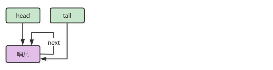
下面以单向环形带哨兵链表方式来实现队列

代码

public class LinkedListQueue<E>
        implements Queue<E>, Iterable<E> {

    private static class Node<E> {
        E value;
        Node<E> next;

        public Node(E value, Node<E> next) {
            this.value = value;
            this.next = next;
        }
    }

    private Node<E> head = new Node<>(null, null);
    private Node<E> tail = head;
    private int size = 0;
    private int capacity = Integer.MAX_VALUE;

    {
        tail.next = head;
    }

    public LinkedListQueue() {
    }

    public LinkedListQueue(int capacity) {
        this.capacity = capacity;
    }

    @Override
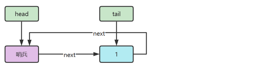
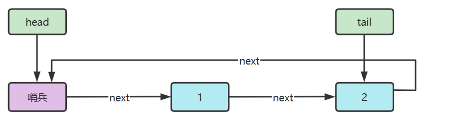
    public boolean offer(E value) {
        if (isFull()) {
            return false;
        }
        Node<E> added = new Node<>(value, head);
        tail.next = added;
        tail = added;
        size++;
        return true;
    }

    @Override
    public E poll() {
        if (isEmpty()) {
            return null;
        }
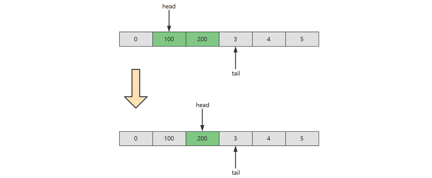
        Node<E> first = head.next;
        head.next = first.next;
        if (first == tail) {
            tail = head;
        }
        size--;
        return first.value;
    }

    @Override
    public E peek() {
        if (isEmpty()) {
            return null;
        }
        return head.next.value;
    }

    @Override
    public boolean isEmpty() {
        return head == tail;
    }

    @Override
    public boolean isFull() {
        return size == capacity;
    }

    @Override
    public Iterator<E> iterator() {
        return new Iterator<E>() {
            Node<E> p = head.next;
            @Override
            public boolean hasNext() {
                return p != head;
            }
            @Override
            public E next() {
                E value = p.value;
                p = p.next;
                return value;
            }
        };
    }
}

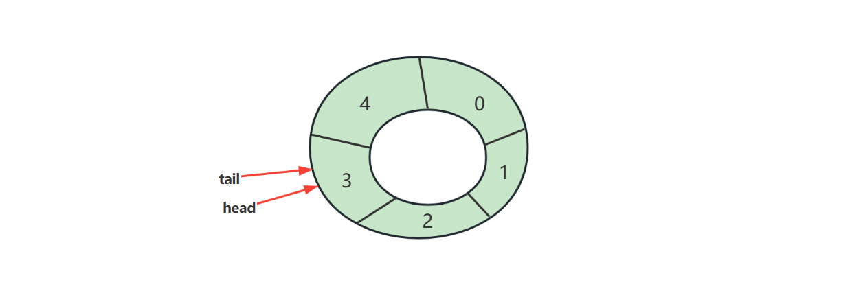
环形数组实现

好处

1. 对比普通数组，起点和终点更为自由，不用考虑数据移动
2. “环”意味着不会存在【越界】问题
3. 数组性能更佳
4. 环形数组比较适合实现有界队列、RingBuffer 等

下标计算

例如，数组长度是 5，当前位置是 3 ，向前走 2 步，此时下标为 $(3+2)\mathrm{\%}5=0$

$$(cur+step)\mathrm{\%}length$$

• cur 当前指针位置
• step 前进步数
• length 数组长度

注意：

• 如果 step = 1，也就是一次走一步，可以在 >= length 时重置为 0 即可

判断空

判断满

满之后的策略可以根据业务需求决定

• 例如我们要实现的环形队列，满之后就拒绝入队

代码

public class ArrayQueue<E> implements Queue<E>, Iterable<E>{

    private int head = 0;
    private int tail = 0;
    private final E[] array;
    private final int length;

    @SuppressWarnings("all")
    public ArrayQueue(int capacity) {
        length = capacity + 1;
        array = (E[]) new Object[length];
    }

    @Override
    public boolean offer(E value) {
        if (isFull()) {
            return false;
        }
        array[tail] = value;
        tail = (tail + 1) % length;
        return true;
    }

    @Override
    public E poll() {
        if (isEmpty()) {
            return null;
        }
        E value = array[head];
        head = (head + 1) % length;
        return value;
    }

    @Override
    public E peek() {
        if (isEmpty()) {
            return null;
        }
        return array[head];
    }

    @Override
    public boolean isEmpty() {
        return tail == head;
    }

    @Override
    public boolean isFull() {
        return (tail + 1) % length == head;
    }

    @Override
    public Iterator<E> iterator() {
        return new Iterator<E>() {
            int p = head;
            @Override
            public boolean hasNext() {
                return p != tail;
            }

            @Override
            public E next() {
                E value = array[p];
                p = (p + 1) % array.length;
                return value;
            }
        };
    }
}

判断空、满方法2

引入 size

public class ArrayQueue2<E> implements Queue<E>, Iterable<E> {

    private int head = 0;
    private int tail = 0;
    private final E[] array;
    private final int capacity;
    private int size = 0;

    @SuppressWarnings("all")
    public ArrayQueue2(int capacity) {
        this.capacity = capacity;
        array = (E[]) new Object[capacity];
    }

    @Override
    public boolean offer(E value) {
        if (isFull()) {
            return false;
        }
        array[tail] = value;
        tail = (tail + 1) % capacity;
        size++;
        return true;
    }

    @Override
    public E poll() {
        if (isEmpty()) {
            return null;
        }
        E value = array[head];
        head = (head + 1) % capacity;
        size--;
        return value;
    }

    @Override
    public E peek() {
        if (isEmpty()) {
            return null;
        }
        return array[head];
    }

    @Override
    public boolean isEmpty() {
        return size == 0;
    }

    @Override
    public boolean isFull() {
        return size == capacity;
    }

    @Override
    public Iterator<E> iterator() {
        return new Iterator<E>() {
            int p = head;

            @Override
            public boolean hasNext() {
                return p != tail;
            }

            @Override
            public E next() {
                E value = array[p];
                p = (p + 1) % capacity;
                return value;
            }
        };
    }
}

判断空、满方法3

• head 和 tail 不断递增，用到索引时，再用它们进行计算，两个问题

  • 如何保证 head 和 tail 自增超过正整数最大值的正确性

  • 如何让取模运算性能更高

• 答案：让 capacity 为 2 的幂

public class ArrayQueue3<E> implements Queue<E>, Iterable<E> {

    private int head = 0;
    private int tail = 0;
    private final E[] array;
    private final int capacity;

    @SuppressWarnings("all")
    public ArrayQueue3(int capacity) {
        if ((capacity & capacity - 1) != 0) {
            throw new IllegalArgumentException("capacity 必须为 2 的幂");
        }
        this.capacity = capacity;
        array = (E[]) new Object[this.capacity];
    }

    @Override
    public boolean offer(E value) {
        if (isFull()) {
            return false;
        }
        array[tail & capacity - 1] = value;
        tail++;
        return true;
    }

    @Override
    public E poll() {
        if (isEmpty()) {
            return null;
        }
        E value = array[head & capacity - 1];
        head++;
        return value;
    }

    @Override
    public E peek() {
        if (isEmpty()) {
            return null;
        }
        return array[head & capacity - 1];
    }

    @Override
    public boolean isEmpty() {
        return tail - head == 0;
    }

    @Override
    public boolean isFull() {
        return tail - head == capacity;
    }

    @Override
    public Iterator<E> iterator() {
        return new Iterator<E>() {
            int p = head;

            @Override
            public boolean hasNext() {
                return p != tail;
            }

            @Override
            public E next() {
                E value = array[p & capacity - 1];
                p++;
                return value;
            }
        };
    }
}

栈

计算机科学中，栈是一种线性的数据结构，只能在其一端添加数据和移除数据。习惯来说，这一端称之为栈顶，另一端不能操作数据的称之为栈底，就如同生活中的一摞书

接口定义

下面定义一个简化的栈接口，规范栈实现过程

public interface Stack<E> {
    /**
     * 向栈顶压入元素
     * @param value 待压入值
     * @return 压入成功返回 true, 否则返回 false
     */
    boolean push(E value);

    /**
     * 从栈顶弹出元素
     * @return 栈非空返回栈顶元素, 栈为空返回 null
     */
    E pop();

    /**
     * 返回栈顶元素, 不弹出
     * @return 栈非空返回栈顶元素, 栈为空返回 null
     */
    E peek();

    /**
     * 判断栈是否为空
     * @return 空返回 true, 否则返回 false
     */
    boolean isEmpty();

    /**
     * 判断栈是否已满
     * @return 满返回 true, 否则返回 false
     */
    boolean isFull();
}

链表实现

public class LinkedListStack<E> implements Stack<E>, Iterable<E> {

    private final int capacity;
    private int size;
    private final Node<E> head = new Node<>(null, null);

    public LinkedListStack(int capacity) {
        this.capacity = capacity;
    }

    @Override
    public boolean push(E value) {
        if (isFull()) {
            return false;
        }
        head.next = new Node<>(value, head.next);
        size++;
        return true;
    }

    @Override
    public E pop() {
        if (isEmpty()) {
            return null;
        }
        Node<E> first = head.next;
        head.next = first.next;
        size--;
        return first.value;
    }

    @Override
    public E peek() {
        if (isEmpty()) {
            return null;
        }
        return head.next.value;
    }

    @Override
    public boolean isEmpty() {
        return head.next == null;
    }

    @Override
    public boolean isFull() {
        return size == capacity;
    }

    @Override
    public Iterator<E> iterator() {
        return new Iterator<E>() {
            Node<E> p = head.next;
            @Override
            public boolean hasNext() {
                return p != null;
            }

            @Override
            public E next() {
                E value = p.value;
                p = p.next;
                return value;
            }
        };
    }

    static class Node<E> {
        E value;
        Node<E> next;

        public Node(E value, Node<E> next) {
            this.value = value;
            this.next = next;
        }
    }
}

数组实现

public class ArrayStack<E> implements Stack<E>, Iterable<E>{
    private final E[] array;
    private int top = 0;

    @SuppressWarnings("all")
    public ArrayStack(int capacity) {
        this.array = (E[]) new Object[capacity];
    }

    @Override
    public boolean push(E value) {
        if (isFull()) {
            return false;
        }
        array[top++] = value;
        return true;
    }

    @Override
    public E pop() {
        if (isEmpty()) {
            return null;
        }
        return array[--top];
    }

    @Override
    public E peek() {
        if (isEmpty()) {
            return null;
        }
        return array[top-1];
    }

    @Override
    public boolean isEmpty() {
        return top == 0;
    }

    @Override
    public boolean isFull() {
        return top == array.length;
    }

    @Override
    public Iterator<E> iterator() {
        return new Iterator<E>() {
            int p = top;
            @Override
            public boolean hasNext() {
                return p > 0;
            }

            @Override
            public E next() {
                return array[--p];
            }
        };
    }
}

应用

模拟如下方法调用

public static void main(String[] args) {
    System.out.println("main1");
    System.out.println("main2");
    method1();
    method2();
    System.out.println("main3");
}

public static void method1() {
    System.out.println("method1");
    method3();
}

public static void method2() {
    System.out.println("method2");
}

public static void method3() {
    System.out.println("method3");
}

模拟代码

public class CPU {
    static class Frame {
        int exit;

        public Frame(int exit) {
            this.exit = exit;
        }
    }
    static int pc = 1; // 模拟程序计数器 Program counter
    static ArrayStack<Frame> stack = new ArrayStack<>(100); // 模拟方法调用栈

    public static void main(String[] args) {
        stack.push(new Frame(-1));
        while (!stack.isEmpty()) {
            switch (pc) {
                case 1 -> {
                    System.out.println("main1");
                    pc++;
                }
                case 2 -> {
                    System.out.println("main2");
                    pc++;
                }
                case 3 -> {
                    stack.push(new Frame(pc + 1));
                    pc = 100;
                }
                case 4 -> {
                    stack.push(new Frame(pc + 1));
                    pc = 200;
                }
                case 5 -> {
                    System.out.println("main3");
                    pc = stack.pop().exit;
                }
                case 100 -> {
                    System.out.println("method1");
                    stack.push(new Frame(pc + 1));
                    pc = 300;
                }
                case 101 -> {
                    pc = stack.pop().exit;
                }
                case 200 -> {
                    System.out.println("method2");
                    pc = stack.pop().exit;
                }
                case 300 -> {
                    System.out.println("method3");
                    pc = stack.pop().exit;
                }
            }
        }
    }
}

双端队列

双端队列（deque，全名double-ended queue）是一种具有队列和栈性质的抽象数据类型。双端队列中的元素可以从两端弹出，插入和删除操作限定在队列的两边进行。

概述

双端队列、队列、栈对比

	定义	特点
队列	一端删除（头）另一端添加（尾）	First In First Out
栈	一端删除和添加（顶）	Last In First Out
双端队列	两端都可以删除、添加
优先级队列		优先级高者先出队
延时队列		根据延时时间确定优先级
并发非阻塞队列	队列空或满时不阻塞
并发阻塞队列	队列空时删除阻塞、队列满时添加阻塞

注1：

• Java 中 LinkedList 即为典型双端队列实现，不过它同时实现了 Queue 接口，也提供了栈的 push pop 等方法

注2：

• 不同语言，操作双端队列的方法命名有所不同，参见下表

  操作	Java	JavaScript	C++	leetCode 641
  尾部插入	offerLast	push	push_back	insertLast
  头部插入	offerFirst	unshift	push_front	insertFront
  尾部移除	pollLast	pop	pop_back	deleteLast
  头部移除	pollFirst	shift	pop_front	deleteFront
  尾部获取	peekLast	at(-1)	back	getRear
  头部获取	peekFirst	at(0)	front	getFront

• 吐槽一下 leetCode 命名比较 low

• 常见的单词还有 enqueue 入队、dequeue 出队

接口定义

public interface Deque<E> {

    boolean offerFirst(E e);

    boolean offerLast(E e);

    E pollFirst();

    E pollLast();

    E peekFirst();

    E peekLast();
    
    boolean isEmpty();

    boolean isFull();
}

链表实现

/**
 * 基于环形链表的双端队列
 * @param <E> 元素类型
 */
public class LinkedListDeque<E> implements Deque<E>, Iterable<E> {

    @Override
    public boolean offerFirst(E e) {
        if (isFull()) {
            return false;
        }
        size++;
        Node<E> a = sentinel;
        Node<E> b = sentinel.next;
        Node<E> offered = new Node<>(a, e, b);
        a.next = offered;
        b.prev = offered;
        return true;
    }

    @Override
    public boolean offerLast(E e) {
        if (isFull()) {
            return false;
        }
        size++;
        Node<E> a = sentinel.prev;
        Node<E> b = sentinel;
        Node<E> offered = new Node<>(a, e, b);
        a.next = offered;
        b.prev = offered;
        return true;
    }

    @Override
    public E pollFirst() {
        if (isEmpty()) {
            return null;
        }
        Node<E> a = sentinel;
        Node<E> polled = sentinel.next;
        Node<E> b = polled.next;
        a.next = b;
        b.prev = a;
        size--;
        return polled.value;
    }

    @Override
    public E pollLast() {
        if (isEmpty()) {
            return null;
        }
        Node<E> polled = sentinel.prev;
        Node<E> a = polled.prev;
        Node<E> b = sentinel;
        a.next = b;
        b.prev = a;
        size--;
        return polled.value;
    }

    @Override
    public E peekFirst() {
        if (isEmpty()) {
            return null;
        }
        return sentinel.next.value;
    }

    @Override
    public E peekLast() {
        if (isEmpty()) {
            return null;
        }
        return sentinel.prev.value;
    }

    @Override
    public boolean isEmpty() {
        return size == 0;
    }

    @Override
    public boolean isFull() {
        return size == capacity;
    }

    @Override
    public Iterator<E> iterator() {
        return new Iterator<E>() {
            Node<E> p = sentinel.next;
            @Override
            public boolean hasNext() {
                return p != sentinel;
            }

            @Override
            public E next() {
                E value = p.value;
                p = p.next;
                return value;
            }
        };
    }

    static class Node<E> {
        Node<E> prev;
        E value;
        Node<E> next;

        public Node(Node<E> prev, E value, Node<E> next) {
            this.prev = prev;
            this.value = value;
            this.next = next;
        }
    }

    Node<E> sentinel = new Node<>(null, null, null);
    int capacity;
    int size;

    public LinkedListDeque(int capacity) {
        sentinel.next = sentinel;
        sentinel.prev = sentinel;
        this.capacity = capacity;
    }
}

数组实现

/**
 * 基于循环数组实现, 特点
 * <ul>
 *     <li>tail 停下来的位置不存储, 会浪费一个位置</li>
 * </ul>
 * @param <E>
 */
public class ArrayDeque1<E> implements Deque<E>, Iterable<E> {

    /*
                    h
            t
        0   1   2   3
        b           a
     */
    @Override
    public boolean offerFirst(E e) {
        if (isFull()) {
            return false;
        }
        head = dec(head, array.length);
        array[head] = e;
        return true;
    }

    @Override
    public boolean offerLast(E e) {
        if (isFull()) {
            return false;
        }
        array[tail] = e;
        tail = inc(tail, array.length);
        return true;
    }

    @Override
    public E pollFirst() {
        if (isEmpty()) {
            return null;
        }
        E e = array[head];
        array[head] = null;
        head = inc(head, array.length);
        return e;
    }

    @Override
    public E pollLast() {
        if (isEmpty()) {
            return null;
        }
        tail = dec(tail, array.length);
        E e = array[tail];
        array[tail] = null;
        return e;
    }

    @Override
    public E peekFirst() {
        if (isEmpty()) {
            return null;
        }
        return array[head];
    }

    @Override
    public E peekLast() {
        if (isEmpty()) {
            return null;
        }
        return array[dec(tail, array.length)];
    }

    @Override
    public boolean isEmpty() {
        return head == tail;
    }

    @Override
    public boolean isFull() {
        if (tail > head) {
            return tail - head == array.length - 1;
        } else if (tail < head) {
            return head - tail == 1;
        } else {
            return false;
        }
    }

    @Override
    public Iterator<E> iterator() {
        return new Iterator<E>() {
            int p = head;
            @Override
            public boolean hasNext() {
                return p != tail;
            }

            @Override
            public E next() {
                E e = array[p];
                p = inc(p, array.length);
                return e;
            }
        };
    }

    E[] array;
    int head;
    int tail;

    @SuppressWarnings("unchecked")
    public ArrayDeque1(int capacity) {
        array = (E[]) new Object[capacity + 1];
    }

    static int inc(int i, int length) {
        if (i + 1 >= length) {
            return 0;
        }
        return i + 1;
    }

    static int dec(int i, int length) {
        if (i - 1 < 0) {
            return length - 1;
        }
        return i - 1;
    }
}

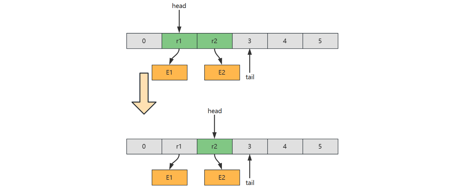
数组实现中，如果存储的是基本类型，那么无需考虑内存释放，例如

但如果存储的是引用类型，应当设置该位置的引用为 null，以便内存及时释放

优先级队列

优先队列（priority queue）是计算机科学中的一类抽象数据类型。优先队列中的每个元素都有各自的优先级，优先级最高的元素最先得到服务；优先级相同的元素按照其在优先队列中的顺序得到服务。优先队列通常使用“堆”（heap）实现。

无序数组实现

要点

1. 入队保持顺序
2. 出队前找到优先级最高的出队，相当于一次选择排序

public class PriorityQueue1<E extends Priority> implements Queue<E> {

    Priority[] array;
    int size;

    public PriorityQueue1(int capacity) {
        array = new Priority[capacity];
    }

    @Override // O(1)
    public boolean offer(E e) {
        if (isFull()) {
            return false;
        }
        array[size++] = e;
        return true;
    }

    // 返回优先级最高的索引值
    private int selectMax() {
        int max = 0;
        for (int i = 1; i < size; i++) {
            if (array[i].priority() > array[max].priority()) {
                max = i;
            }
        }
        return max;
    }

    @Override // O(n)
    public E poll() {
        if (isEmpty()) {
            return null;
        }
        int max = selectMax();
        E e = (E) array[max];
        remove(max);
        return e;
    }

    private void remove(int index) {
        if (index < size - 1) {
            System.arraycopy(array, index + 1,
                    array, index, size - 1 - index);
        }
        array[--size] = null; // help GC
    }

    @Override
    public E peek() {
        if (isEmpty()) {
            return null;
        }
        int max = selectMax();
        return (E) array[max];
    }

    @Override
    public boolean isEmpty() {
        return size == 0;
    }

    @Override
    public boolean isFull() {
        return size == array.length;
    }
}

有序数组实现

要点

1. 入队后排好序，优先级最高的排列在尾部
2. 出队只需删除尾部元素即可

public class PriorityQueue2<E extends Priority> implements Queue<E> {

    Priority[] array;
    int size;

    public PriorityQueue2(int capacity) {
        array = new Priority[capacity];
    }

    // O(n)
    @Override
    public boolean offer(E e) {
        if (isFull()) {
            return false;
        }
        insert(e);
        size++;
        return true;
    }

    // 一轮插入排序
    private void insert(E e) {
        int i = size - 1;
        while (i >= 0 && array[i].priority() > e.priority()) {
            array[i + 1] = array[i];
            i--;
        }
        array[i + 1] = e;
    }

    // O(1)
    @Override
    public E poll() {
        if (isEmpty()) {
            return null;
        }
        E e = (E) array[size - 1];
        array[--size] = null; // help GC
        return e;
    }

    @Override
    public E peek() {
        if (isEmpty()) {
            return null;
        }
        return (E) array[size - 1];
    }

    @Override
    public boolean isEmpty() {
        return size == 0;
    }

    @Override
    public boolean isFull() {
        return size == array.length;
    }
}

堆实现

计算机科学中，堆是一种基于树的数据结构，通常用完全二叉树实现。堆的特性如下

• 在大顶堆中，任意节点 C 与它的父节点 P 符合 $P.value\ge C.value$
• 而小顶堆中，任意节点 C 与它的父节点 P 符合 $P.value\le C.value$
• 最顶层的节点（没有父亲）称之为 root 根节点

In computer science, a heap is a specialized tree-based data structure which is essentially an almost complete tree that satisfies the heap property: in a max heap, for any given node C, if P is a parent node of C, then the key (the value) of P is greater than or equal to the key of C. In a min heap, the key of P is less than or equal to the key of C. The node at the "top" of the heap (with no parents) is called the root node

例1 - 满二叉树（Full Binary Tree）特点：每一层都是填满的

例2 - 完全二叉树（Complete Binary Tree）特点：最后一层可能未填满，靠左对齐

例3 - 大顶堆

例4 - 小顶堆

完全二叉树可以使用数组来表示

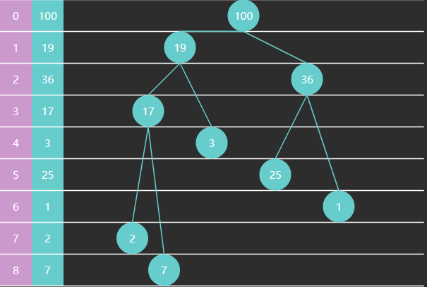
特征

• 如果从索引 0 开始存储节点数据
  • 节点 $i$ 的父节点为 $floor((i-1)/2)$，当 $i>0$ 时
  • 节点 $i$ 的左子节点为 $2i+1$，右子节点为 $2i+2$，当然它们得 $<size$
• 如果从索引 1 开始存储节点数据
  • 节点 $i$ 的父节点为 $floor(i/2)$，当 $i>1$ 时
  • 节点 $i$ 的左子节点为 $2i$，右子节点为 $2i+1$，同样得 $<size$

代码

public class PriorityQueue4<E extends Priority> implements Queue<E> {

    Priority[] array;
    int size;

    public PriorityQueue4(int capacity) {
        array = new Priority[capacity];
    }

    @Override
    public boolean offer(E offered) {
        if (isFull()) {
            return false;
        }
        int child = size++;
        int parent = (child - 1) / 2;
        while (child > 0 && offered.priority() > array[parent].priority()) {
            array[child] = array[parent];
            child = parent;
            parent = (child - 1) / 2;
        }
        array[child] = offered;
        return true;
    }


    private void swap(int i, int j) {
        Priority t = array[i];
        array[i] = array[j];
        array[j] = t;
    }

    @Override
    public E poll() {
        if (isEmpty()) {
            return null;
        }
        swap(0, size - 1);
        size--;
        Priority e = array[size];
        array[size] = null;
        
        shiftDown(0);        
        return (E) e;
    }

    void shiftDown(int parent) {
        int left = 2 * parent + 1;
        int right = left + 1;
        int max = parent;
        if (left < size && array[left].priority() > array[max].priority()) {
            max = left;
        }
        if (right < size && array[right].priority() > array[max].priority()) {
            max = right;
        }
        if (max != parent) {
            swap(max, parent);
            shiftDown(max);
        }
    }

    @Override
    public E peek() {
        if (isEmpty()) {
            return null;
        }
        return (E) array[0];
    }

    @Override
    public boolean isEmpty() {
        return size == 0;
    }

    @Override
    public boolean isFull() {
        return size == array.length;
    }
}

阻塞队列

阻塞队列（BlockingQueue） 是一个支持两个附加操作的队列。这两个附加的操作是：在队列为空时，获取元素的线程会等待队列变为非空。当队列满时，存储元素的线程会等待队列可用。阻塞队列常用于生产者和消费者的场景，生产者是往队列里添加元素的线程，消费者是从队列里拿元素的线程。阻塞队列就是生产者存放元素的容器，而消费者也只从容器里拿元素。

概述

之前的队列在很多场景下都不能很好地工作，例如

1. 大部分场景要求分离向队列放入（生产者）、从队列拿出（消费者）两个角色、它们得由不同的线程来担当，而之前的实现根本没有考虑线程安全问题
2. 队列为空，那么在之前的实现里会返回 null，如果就是硬要拿到一个元素呢？只能不断循环尝试
3. 队列为满，那么再之前的实现里会返回 false，如果就是硬要塞入一个元素呢？只能不断循环尝试

因此我们需要解决的问题有

1. 用锁保证线程安全
2. 用条件变量让等待非空线程与等待不满线程进入等待状态，而不是不断循环尝试，让 CPU 空转

有同学对线程安全还没有足够的认识，下面举一个反例，两个线程都要执行入队操作（几乎在同一时刻）

public class TestThreadUnsafe {
    private final String[] array = new String[10];
    private int tail = 0;

    public void offer(String e) {
        array[tail] = e;
        tail++;
    }

    @Override
    public String toString() {
        return Arrays.toString(array);
    }

    public static void main(String[] args) {
        TestThreadUnsafe queue = new TestThreadUnsafe();
        new Thread(()-> queue.offer("e1"), "t1").start();
        new Thread(()-> queue.offer("e2"), "t2").start();
    }
}

执行的时间序列如下，假设初始状态 tail = 0，在执行过程中由于 CPU 在两个线程之间切换，造成了指令交错

线程1	线程2	说明
array[tail]=e1		线程1 向 tail 位置加入 e1 这个元素，但还没来得及执行 tail++
	array[tail]=e2	线程2 向 tail 位置加入 e2 这个元素，覆盖掉了 e1
	tail++	tail 自增为1
tail++		tail 自增为2
		最后状态 tail 为 2，数组为 [e2, null, null ...]

糟糕的是，由于指令交错的顺序不同，得到的结果不止以上一种，宏观上造成混乱的效果

单锁实现

Java 中要防止代码段交错执行，需要使用锁，有两种选择

• synchronized 代码块，属于关键字级别提供锁保护，功能少
• ReentrantLock 类，功能丰富

以 ReentrantLock 为例

ReentrantLock lock = new ReentrantLock();

public void offer(String e) {
    lock.lockInterruptibly();
    try {
        array[tail] = e;
        tail++;
    } finally {
        lock.unlock();
    }
}

只要两个线程执行上段代码时，锁对象是同一个，就能保证 try 块内的代码的执行不会出现指令交错现象，即执行顺序只可能是下面两种情况之一

线程1	线程2	说明
lock.lockInterruptibly()		t1对锁对象上锁
array[tail]=e1
	lock.lockInterruptibly()	即使 CPU 切换到线程2，但由于t1已经对该对象上锁，因此线程2卡在这儿进不去
tail++		切换回线程1 执行后续代码
lock.unlock()		线程1 解锁
	array[tail]=e2	线程2 此时才能获得锁，执行它的代码
	tail++

• 另一种情况是线程2 先获得锁，线程1 被挡在外面
• 要明白保护的本质，本例中是保护的是 tail 位置读写的安全

事情还没有完，上面的例子是队列还没有放满的情况，考虑下面的代码（这回锁同时保护了 tail 和 size 的读写安全）

ReentrantLock lock = new ReentrantLock();
int size = 0;

public void offer(String e) {
    lock.lockInterruptibly();
    try {
        if(isFull()) {
            // 满了怎么办?
        }
        array[tail] = e;
        tail++;
        
        size++;
    } finally {
        lock.unlock();
    }
}

private boolean isFull() {
    return size == array.length;
}

之前是返回 false 表示添加失败，前面分析过想达到这么一种效果：

• 在队列满时，不是立刻返回，而是当前线程进入等待
• 什么时候队列不满了，再唤醒这个等待的线程，从上次的代码处继续向下运行

ReentrantLock 可以配合条件变量来实现，代码进化为

ReentrantLock lock = new ReentrantLock();
Condition tailWaits = lock.newCondition(); // 条件变量
int size = 0;

public void offer(String e) {
    lock.lockInterruptibly();
    try {
        while (isFull()) {
            tailWaits.await();	// 当队列满时, 当前线程进入 tailWaits 等待
        }
        array[tail] = e;
        tail++;
        
        size++;
    } finally {
        lock.unlock();
    }
}

private boolean isFull() {
    return size == array.length;
}

• 条件变量底层也是个队列，用来存储这些需要等待的线程，当队列满了，就会将 offer 线程加入条件队列，并暂时释放锁
• 将来我们的队列如果不满了（由 poll 线程那边得知）可以调用 tailWaits.signal() 来唤醒 tailWaits 中首个等待的线程，被唤醒的线程会再次抢到锁，从上次 await 处继续向下运行

思考为何要用 while 而不是 if，设队列容量是 3

操作前	offer(4)	offer(5)	poll()	操作后
[1 2 3]	队列满，进入tailWaits 等待			[1 2 3]
[1 2 3]			取走 1，队列不满，唤醒线程	[2 3]
[2 3]		抢先获得锁，发现不满，放入 5		[2 3 5]
[2 3 5]	从上次等待处直接向下执行			[2 3 5 ?]

关键点：

• 从 tailWaits 中唤醒的线程，会与新来的 offer 的线程争抢锁，谁能抢到是不一定的，如果后者先抢到，就会导致条件又发生变化
• 这种情况称之为虚假唤醒，唤醒后应该重新检查条件，看是不是得重新进入等待

最后的实现代码

/**
 * 单锁实现
 * @param <E> 元素类型
 */
public class BlockingQueue1<E> implements BlockingQueue<E> {
    private final E[] array;
    private int head = 0;
    private int tail = 0;
    private int size = 0; // 元素个数

    @SuppressWarnings("all")
    public BlockingQueue1(int capacity) {
        array = (E[]) new Object[capacity];
    }

    ReentrantLock lock = new ReentrantLock();
    Condition tailWaits = lock.newCondition();
    Condition headWaits = lock.newCondition();

    @Override
    public void offer(E e) throws InterruptedException {
        lock.lockInterruptibly();
        try {
            while (isFull()) {
                tailWaits.await();
            }
            array[tail] = e;
            if (++tail == array.length) {
                tail = 0;
            }
            size++;
            headWaits.signal();
        } finally {
            lock.unlock();
        }
    }

    @Override
    public void offer(E e, long timeout) throws InterruptedException {
        lock.lockInterruptibly();
        try {
            long t = TimeUnit.MILLISECONDS.toNanos(timeout);
            while (isFull()) {
                if (t <= 0) {
                    return;
                }
                t = tailWaits.awaitNanos(t);
            }
            array[tail] = e;
            if (++tail == array.length) {
                tail = 0;
            }
            size++;
            headWaits.signal();
        } finally {
            lock.unlock();
        }
    }

    @Override
    public E poll() throws InterruptedException {
        lock.lockInterruptibly();
        try {
            while (isEmpty()) {
                headWaits.await();
            }
            E e = array[head];
            array[head] = null; // help GC
            if (++head == array.length) {
                head = 0;
            }
            size--;
            tailWaits.signal();
            return e;
        } finally {
            lock.unlock();
        }
    }

    private boolean isEmpty() {
        return size == 0;
    }

    private boolean isFull() {
        return size == array.length;
    }
}

• public void offer(E e, long timeout) throws InterruptedException 是带超时的版本，可以只等待一段时间，而不是永久等下去，类似的 poll 也可以做带超时的版本，这个留给大家了

注意

• JDK 中 BlockingQueue 接口的方法命名与我的示例有些差异
  • 方法 offer(E e) 是非阻塞的实现，阻塞实现方法为 put(E e)
  • 方法 poll() 是非阻塞的实现，阻塞实现方法为 take()

双锁实现

单锁的缺点在于：

• 生产和消费几乎是不冲突的，唯一冲突的是生产者和消费者它们有可能同时修改 size
• 冲突的主要是生产者之间：多个 offer 线程修改 tail
• 冲突的还有消费者之间：多个 poll 线程修改 head

如果希望进一步提高性能，可以用两把锁

• 一把锁保护 tail
• 另一把锁保护 head

ReentrantLock headLock = new ReentrantLock();  // 保护 head 的锁
Condition headWaits = headLock.newCondition(); // 队列空时，需要等待的线程集合

ReentrantLock tailLock = new ReentrantLock();  // 保护 tail 的锁
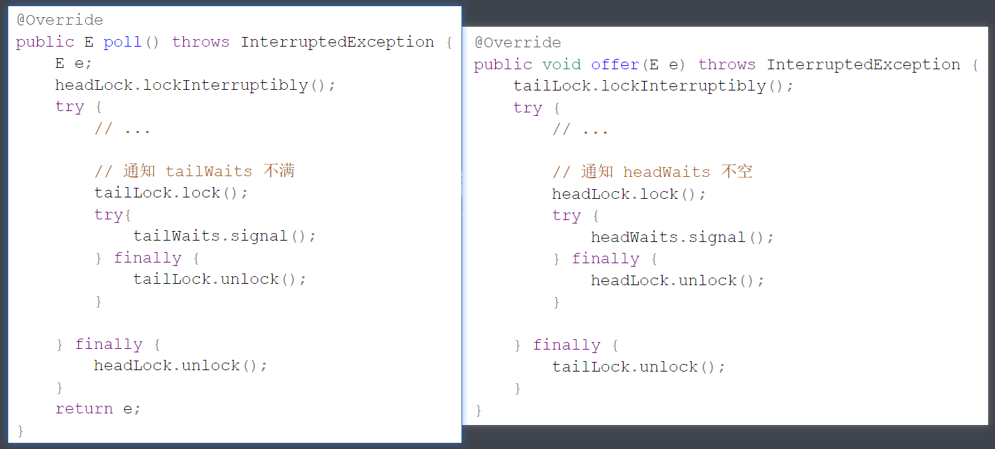
Condition tailWaits = tailLock.newCondition(); // 队列满时，需要等待的线程集合

先看看 offer 方法的初步实现

@Override
public void offer(E e) throws InterruptedException {
    tailLock.lockInterruptibly();
    try {
        // 队列满等待
        while (isFull()) {
            tailWaits.await();
        }
        
        // 不满则入队
        array[tail] = e;
        if (++tail == array.length) {
            tail = 0;
        }
        
        // 修改 size （有问题）
        size++;
        
    } finally {
        tailLock.unlock();
    }
}

上面代码的缺点是 size 并不受 tailLock 保护，tailLock 与 headLock 是两把不同的锁，并不能实现互斥的效果。因此，size 需要用下面的代码保证原子性

AtomicInteger size = new AtomicInteger(0);	   // 保护 size 的原子变量

size.getAndIncrement(); // 自增
size.getAndDecrement(); // 自减

代码修改为

@Override
public void offer(E e) throws InterruptedException {
    tailLock.lockInterruptibly();
    try {
        // 队列满等待
        while (isFull()) {
            tailWaits.await();
        }
        
        // 不满则入队
        array[tail] = e;
        if (++tail == array.length) {
            tail = 0;
        }
        
        // 修改 size
        size.getAndIncrement();
        
    } finally {
        tailLock.unlock();
    }
}

对称地，可以写出 poll 方法

@Override
public E poll() throws InterruptedException {
    E e;
    headLock.lockInterruptibly();
    try {
        // 队列空等待
        while (isEmpty()) {
            headWaits.await();
        }
        
        // 不空则出队
        e = array[head];
        if (++head == array.length) {
            head = 0;
        }
        
        // 修改 size
        size.getAndDecrement();
        
    } finally {
        headLock.unlock();
    }
    return e;
}

下面来看一个难题，就是如何通知 headWaits 和 tailWaits 中等待的线程，比如 poll 方法拿走一个元素，通知 tailWaits：我拿走一个，不满了噢，你们可以放了，因此代码改为

@Override
public E poll() throws InterruptedException {
    E e;
    headLock.lockInterruptibly();
    try {
        // 队列空等待
        while (isEmpty()) {
            headWaits.await();
        }
        
        // 不空则出队
        e = array[head];
        if (++head == array.length) {
            head = 0;
        }
        
        // 修改 size
        size.getAndDecrement();
        
        // 通知 tailWaits 不满（有问题）
        tailWaits.signal();
        
    } finally {
        headLock.unlock();
    }
    return e;
}

问题在于要使用这些条件变量的 await()， signal() 等方法需要先获得与之关联的锁，上面的代码若直接运行会出现以下错误

java.lang.IllegalMonitorStateException

那有同学说，加上锁不就行了吗，于是写出了下面的代码

发现什么问题了？两把锁这么嵌套使用，非常容易出现死锁，如下所示

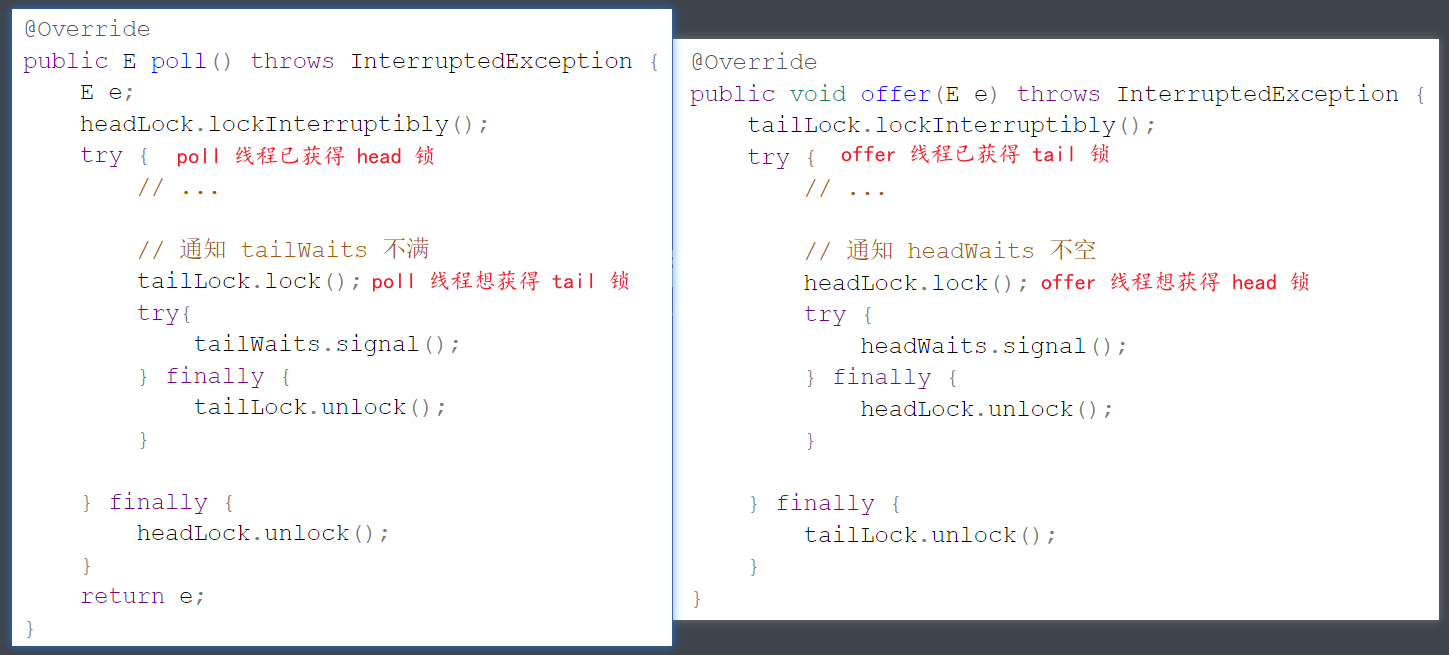
因此得避免嵌套，两段加锁的代码变成了下面平级的样子

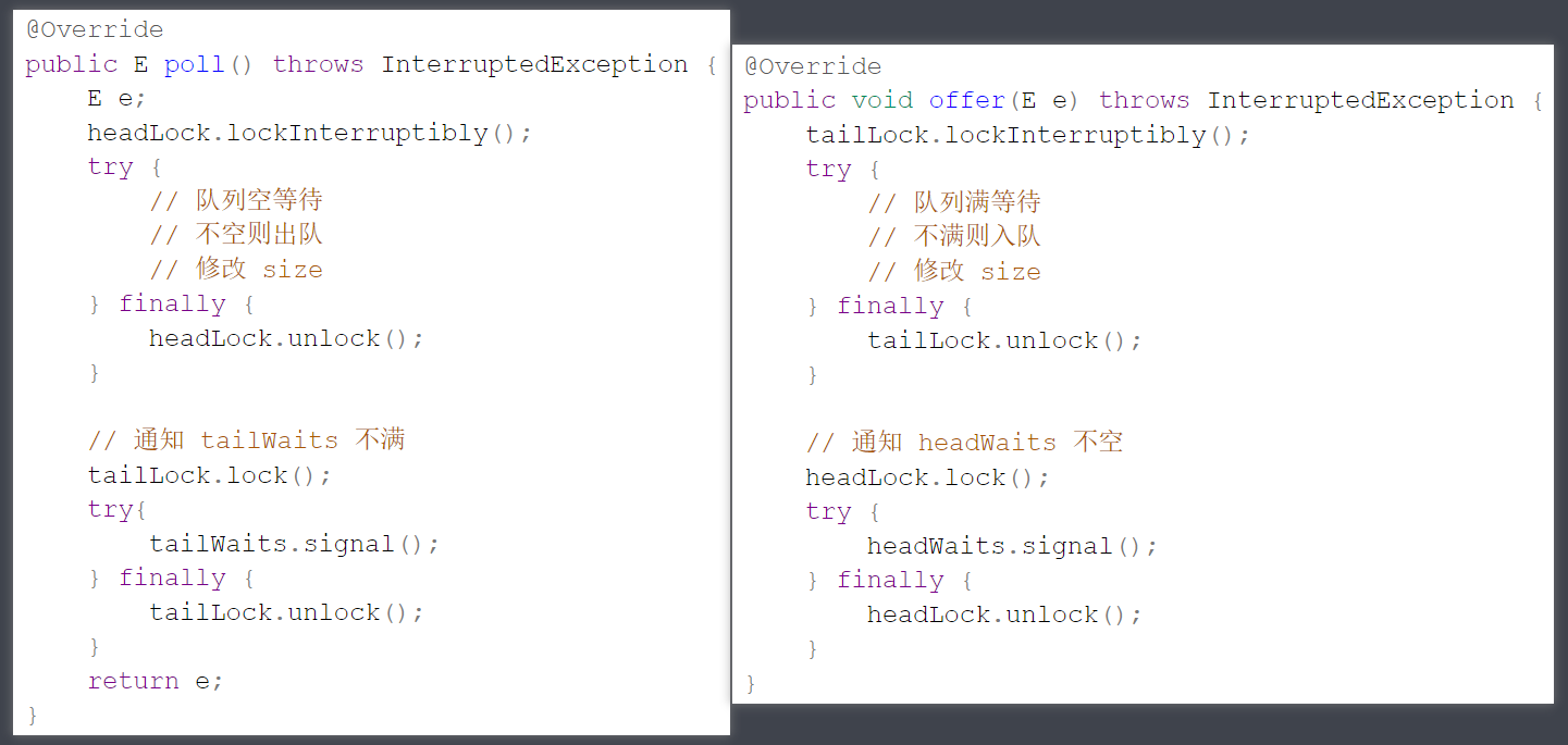
性能还可以进一步提升

1. 代码调整后 offer 并没有同时获取 tailLock 和 headLock 两把锁，因此两次加锁之间会有空隙，这个空隙内可能有其它的 offer 线程添加了更多的元素，那么这些线程都要执行 signal()，通知 poll 线程队列非空吗？

   • 每次调用 signal() 都需要这些 offer 线程先获得 headLock 锁，成本较高，要想法减少 offer 线程获得 headLock 锁的次数
   • 可以加一个条件：当 offer 增加前队列为空，即从 0 变化到不空，才由此 offer 线程来通知 headWaits，其它情况不归它管

2. 队列从 0 变化到不空，会唤醒一个等待的 poll 线程，这个线程被唤醒后，肯定能拿到 headLock 锁，因此它具备了唤醒 headWaits 上其它 poll 线程的先决条件。如果检查出此时有其它 offer 线程新增了元素（不空，但不是从0变化而来），那么不妨由此 poll 线程来唤醒其它 poll 线程

这个技巧被称之为级联通知（cascading notifies），类似的原因

3. 在 poll 时队列从满变化到不满，才由此 poll 线程来唤醒一个等待的 offer 线程，目的也是为了减少 poll 线程对 tailLock 上锁次数，剩下等待的 offer 线程由这个 offer 线程间接唤醒

最终的代码为

public class BlockingQueue2<E> implements BlockingQueue<E> {

    private final E[] array;
    private int head = 0;
    private int tail = 0;
    private final AtomicInteger size = new AtomicInteger(0);
    ReentrantLock headLock = new ReentrantLock();
    Condition headWaits = headLock.newCondition();
    ReentrantLock tailLock = new ReentrantLock();
    Condition tailWaits = tailLock.newCondition();

    public BlockingQueue2(int capacity) {
        this.array = (E[]) new Object[capacity];
    }

    @Override
    public void offer(E e) throws InterruptedException {
        int c;
        tailLock.lockInterruptibly();
        try {
            while (isFull()) {
                tailWaits.await();
            }
            array[tail] = e;
            if (++tail == array.length) {
                tail = 0;
            }            
            c = size.getAndIncrement();
            // a. 队列不满, 但不是从满->不满, 由此offer线程唤醒其它offer线程
            if (c + 1 < array.length) {
                tailWaits.signal();
            }
        } finally {
            tailLock.unlock();
        }
        // b. 从0->不空, 由此offer线程唤醒等待的poll线程
        if (c == 0) {
            headLock.lock();
            try {
                headWaits.signal();
            } finally {
                headLock.unlock();
            }
        }
    }

    @Override
    public E poll() throws InterruptedException {
        E e;
        int c;
        headLock.lockInterruptibly();
        try {
            while (isEmpty()) {
                headWaits.await(); 
            }
            e = array[head]; 
            if (++head == array.length) {
                head = 0;
            }
            c = size.getAndDecrement();
            // b. 队列不空, 但不是从0变化到不空，由此poll线程通知其它poll线程
            if (c > 1) {
                headWaits.signal();
            }
        } finally {
            headLock.unlock();
        }
        // a. 从满->不满, 由此poll线程唤醒等待的offer线程
        if (c == array.length) {
            tailLock.lock();
            try {
                tailWaits.signal();
            } finally {
                tailLock.unlock();
            }
        }
        return e;
    }

    private boolean isEmpty() {
        return size.get() == 0;
    }

    private boolean isFull() {
        return size.get() == array.length;
    }

}

双锁实现的非常精巧，据说作者 Doug Lea 花了一年的时间才完善了此段代码

堆

堆（Heap）是计算机科学中的一种特别的完全二叉树。若是满足以下特性，即可称为堆：“给定堆中任意节点P和C，若P是C的母节点，那么P的值会小于等于（或大于等于）C的值”。若母节点的值恒小于等于子节点的值，此堆称为最小堆（min heap）；反之，若母节点的值恒大于等于子节点的值，此堆称为最大堆（max heap）。在堆中最顶端的那一个节点，称作根节点（root node），根节点本身没有父节点（parent node）。

堆始于J. W. J. Williams在1964年发表的堆排序（heap sort），当时他提出了二叉堆树作为此算法的数据结构。

实现

以大顶堆为例，相对于之前的优先级队列，增加了堆化等方法

public class MaxHeap {
    int[] array;
    int size;

    public MaxHeap(int capacity) {
        this.array = new int[capacity];
    }

    /**
     * 获取堆顶元素
     *
     * @return 堆顶元素
     */
    public int peek() {
        return array[0];
    }

    /**
     * 删除堆顶元素
     *
     * @return 堆顶元素
     */
    public int poll() {
        int top = array[0];
        swap(0, size - 1);
        size--;
        down(0);
        return top;
    }

    /**
     * 删除指定索引处元素
     *
     * @param index 索引
     * @return 被删除元素
     */
    public int poll(int index) {
        int deleted = array[index];
        up(Integer.MAX_VALUE, index);
        poll();
        return deleted;
    }

    /**
     * 替换堆顶元素
     *
     * @param replaced 新元素
     */
    public void replace(int replaced) {
        array[0] = replaced;
        down(0);
    }

    /**
     * 堆的尾部添加元素
     *
     * @param offered 新元素
     * @return 是否添加成功
     */
    public boolean offer(int offered) {
        if (size == array.length) {
            return false;
        }
        up(offered, size);
        size++;
        return true;
    }

    // 将 offered 元素上浮: 直至 offered 小于父元素或到堆顶
    private void up(int offered, int index) {
        int child = index;
        while (child > 0) {
            int parent = (child - 1) / 2;
            if (offered > array[parent]) {
                array[child] = array[parent];
            } else {
                break;
            }
            child = parent;
        }
        array[child] = offered;
    }

    public MaxHeap(int[] array) {
        this.array = array;
        this.size = array.length;
        heapify();
    }

    // 建堆
    private void heapify() {
        // 如何找到最后这个非叶子节点  size / 2 - 1
        for (int i = size / 2 - 1; i >= 0; i--) {
            down(i);
        }
    }

    // 将 parent 索引处的元素下潜: 与两个孩子较大者交换, 直至没孩子或孩子没它大
    private void down(int parent) {
        int left = parent * 2 + 1;
        int right = left + 1;
        int max = parent;
        if (left < size && array[left] > array[max]) {
            max = left;
        }
        if (right < size && array[right] > array[max]) {
            max = right;
        }
        if (max != parent) { // 找到了更大的孩子
            swap(max, parent);
            down(max);
        }
    }

    // 交换两个索引处的元素
    private void swap(int i, int j) {
        int t = array[i];
        array[i] = array[j];
        array[j] = t;
    }

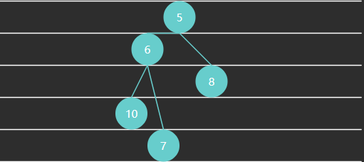
    public static void main(String[] args) {

        int[] array = {2, 3, 1, 7, 6, 4, 5};
        MaxHeap heap = new MaxHeap(array);
        System.out.println(Arrays.toString(heap.array));

        while (heap.size > 1) {
            heap.swap(0, heap.size - 1);
            heap.size--;
            heap.down(0);
        }

        System.out.println(Arrays.toString(heap.array));
    }
}

建堆算法

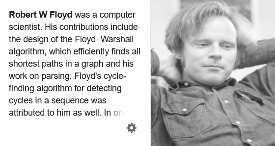
Floyd 建堆算法作者（也是之前龟兔赛跑判环作者）：

1. 找到最后一个非叶子节点
2. 从后向前，对每个节点执行下潜

一些规律

• 一棵满二叉树节点个数为 $2^h-1$，如下例中高度 $h=3$ 节点数是 $2^3-1=7$
• 非叶子节点范围为 $[0,size/2-1]$

算法时间复杂度分析

下面看交换次数的推导：设节点高度为 3

	本层节点数	高度	下潜最多交换次数（高度-1）
4567 这层	4	1	0
23这层	2	2	1
1这层	1	3	2

每一层的交换次数为：$\mathrm{节}\mathrm{点}\mathrm{个}\mathrm{数}\ast \mathrm{此}\mathrm{节}\mathrm{点}\mathrm{交}\mathrm{换}\mathrm{次}\mathrm{数}$，总的交换次数为

$$\begin{array}{rl}& 4\ast 0+2\ast 1+1\ast 2\\ & \frac{8}{2}\ast 0+\frac{8}{4}\ast 1+\frac{8}{8}\ast 2\\ & \frac{8}{2^1}\ast 0+\frac{8}{2^2}\ast 1+\frac{8}{2^3}\ast 2\end{array}$$

即

$$\sum _{i=1}^h(\frac{2^h}{2^i}\ast (i-1))$$

在 https://www.wolframalpha.com/ 输入

Sum[\(40)Divide[Power[2,x],Power[2,i]]*\(40)i-1\(41)\(41),{i,1,x}]

推导出

$$2^h-h-1$$

其中 $2^h\approx n$，$h\approx {\log }_{2}n$，因此有时间复杂度 $O(n)$

二叉树

在计算机科学中，二叉树（英语：Binary tree）是每个节点最多只有两个分支（即不存在分支度大于2的节点）的树结构[1]。通常分支被称作“左子树”或“右子树”。二叉树的分支具有左右次序，不能随意颠倒。

概述

重要的二叉树结构

• 完全二叉树（complete binary tree）是一种二叉树结构，除最后一层以外，每一层都必须填满，填充时要遵从先左后右
• 平衡二叉树（balance binary tree）是一种二叉树结构，其中每个节点的左右子树高度相差不超过 1

存储

存储方式分为两种

1. 定义树节点与左、右孩子引用（TreeNode）
2. 使用数组，前面讲堆时用过，若以 0 作为树的根，索引可以通过如下方式计算
   • 父 = floor((子 - 1) / 2)
   • 左孩子 = 父 * 2 + 1
   • 右孩子 = 父 * 2 + 2

遍历

遍历也分为两种

1. 广度优先遍历（Breadth-first order）：尽可能先访问距离根最近的节点，也称为层序遍历
2. 深度优先遍历（Depth-first order）：对于二叉树，可以进一步分成三种（要深入到叶子节点）
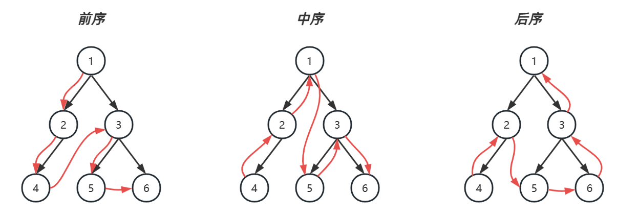
   1. pre-order 前序遍历，对于每一棵子树，先访问该节点，然后是左子树，最后是右子树
   2. in-order 中序遍历，对于每一棵子树，先访问左子树，然后是该节点，最后是右子树
   3. post-order 后序遍历，对于每一棵子树，先访问左子树，然后是右子树，最后是该节点

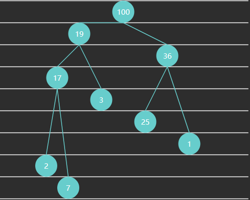
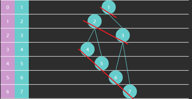
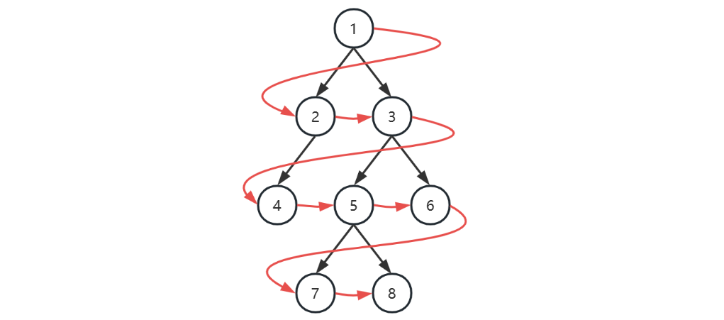
广度优先

本轮开始时队列	本轮访问节点
[1]	1
[2, 3]	2
[3, 4]	3
[4, 5, 6]	4
[5, 6]	5
[6, 7, 8]	6
[7, 8]	7
[8]	8
[]

1. 初始化，将根节点加入队列
2. 循环处理队列中每个节点，直至队列为空
3. 每次循环内处理节点后，将它的孩子节点（即下一层的节点）加入队列

注意

• 以上用队列来层序遍历是针对 TreeNode 这种方式表示的二叉树

• 对于数组表现的二叉树，则直接遍历数组即可，自然为层序遍历的顺序

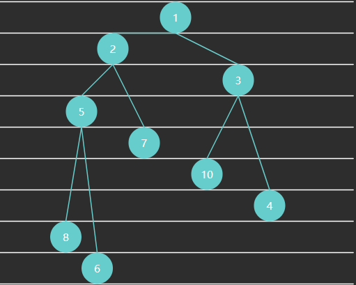
深度优先

栈暂存	已处理	前序遍历	中序遍历
[1]	1 ✔️ 左💤 右💤	1
[1, 2]	2✔️ 左💤 右💤 1✔️ 左💤 右💤	2
[1, 2, 4]	4✔️ 左✔️ 右✔️ 2✔️ 左💤 右💤 1✔️ 左💤 右💤	4	4
[1, 2]	2✔️ 左✔️ 右✔️ 1✔️ 左💤 右💤		2
[1]	1✔️ 左✔️ 右💤		1
[1, 3]	3✔️ 左💤 右💤 1✔️ 左✔️ 右💤	3
[1, 3, 5]	5✔️ 左✔️ 右✔️ 3✔️ 左💤 右💤 1✔️ 左✔️ 右💤	5	5
[1, 3]	3✔️ 左✔️ 右💤 1✔️ 左✔️ 右💤		3
[1, 3, 6]	6✔️ 左✔️ 右✔️ 3✔️ 左✔️ 右💤 1✔️ 左✔️ 右💤	6	6
[1, 3]	3✔️ 左✔️ 右✔️ 1✔️ 左✔️ 右💤
[1]	1✔️ 左✔️ 右✔️
[]

递归实现

/**
 * <h3>前序遍历</h3>
 * @param node 节点
 */
static void preOrder(TreeNode node) {
    if (node == null) {
        return;
    }
    System.out.print(node.val + "\t"); // 值
    preOrder(node.left); // 左
    preOrder(node.right); // 右
}

/**
 * <h3>中序遍历</h3>
 * @param node 节点
 */
static void inOrder(TreeNode node) {
    if (node == null) {
        return;
    }
    inOrder(node.left); // 左
    System.out.print(node.val + "\t"); // 值
    inOrder(node.right); // 右
}

/**
 * <h3>后序遍历</h3>
 * @param node 节点
 */
static void postOrder(TreeNode node) {
    if (node == null) {
        return;
    }
    postOrder(node.left); // 左
    postOrder(node.right); // 右
    System.out.print(node.val + "\t"); // 值
}

非递归实现

前序遍历

LinkedListStack<TreeNode> stack = new LinkedListStack<>();
TreeNode curr = root;

while (!stack.isEmpty() || curr != null) {
    if (curr != null) {
        stack.push(curr);
        System.out.println(curr);
        curr = curr.left;
    } else {
        TreeNode pop = stack.pop();
        curr = pop.right;
    }

}

中序遍历

LinkedListStack<TreeNode> stack = new LinkedListStack<>();
TreeNode curr = root;

while (!stack.isEmpty() || curr != null) {
    if (curr != null) {
        stack.push(curr);
        curr = curr.left;
    } else {
        TreeNode pop = stack.pop();
        System.out.println(pop);
        curr = pop.right;
    }
}

后序遍历

LinkedListStack<TreeNode> stack = new LinkedListStack<>();
TreeNode curr = root;
TreeNode pop = null;

while (!stack.isEmpty() || curr != null) {
    if (curr != null) {
        stack.push(curr);
        curr = curr.left;
    } else {
        TreeNode peek = stack.peek();
        if (peek.right == null || peek.right == pop) {
            pop = stack.pop();
            System.out.println(pop);
        } else {
            curr = peek.right;
        }
    }
}

对于后序遍历，向回走时，需要处理完右子树才能 pop 出栈。如何知道右子树处理完成呢？

• 如果栈顶元素的 $right\equiv null$ 表示没啥可处理的，可以出栈

• 如果栈顶元素的 $right\ne null$，

  • 那么使用 lastPop 记录最近出栈的节点，即表示从这个节点向回走
  • 如果栈顶元素的 $right==lastPop$ 此时应当出栈

对于前、中两种遍历，实际以上代码从右子树向回走时，并未走完全程（stack 提前出栈了）后序遍历以上代码是走完全程了

统一写法

下面是一种统一的写法，依据后序遍历修改

LinkedList<TreeNode> stack = new LinkedList<>();

TreeNode curr = root; // 代表当前节点
TreeNode pop = null; // 最近一次弹栈的元素
while (curr != null || !stack.isEmpty()) {
    if (curr != null) {
        colorPrintln("前: " + curr.val, 31);
        stack.push(curr); // 压入栈，为了记住回来的路
        curr = curr.left;
    } else {
        TreeNode peek = stack.peek();
        // 右子树可以不处理, 对中序来说, 要在右子树处理之前打印
        if (peek.right == null) {
            colorPrintln("中: " + peek.val, 36);
            pop = stack.pop();
            colorPrintln("后: " + pop.val, 34);
        }
        // 右子树处理完成, 对中序来说, 无需打印
        else if (peek.right == pop) {
            pop = stack.pop();
            colorPrintln("后: " + pop.val, 34);
        }
        // 右子树待处理, 对中序来说, 要在右子树处理之前打印
        else {
            colorPrintln("中: " + peek.val, 36);
            curr = peek.right;
        }
    }
}

public static void colorPrintln(String origin, int color) {
    System.out.printf("\033[%dm%s\033[0m%n", color, origin);
}

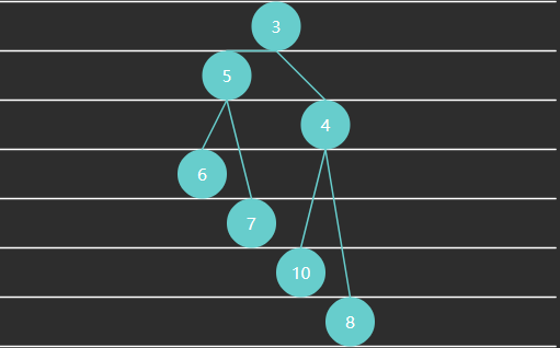
一张图演示三种遍历

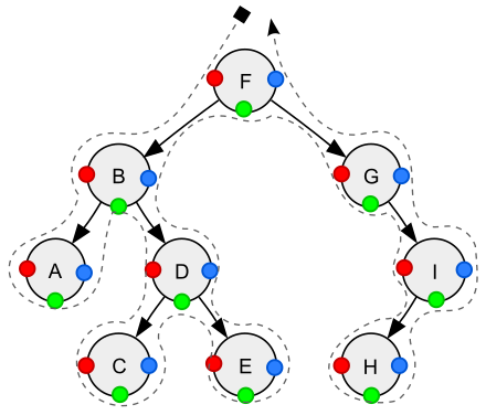
• 红色：前序遍历顺序
• 绿色：中序遍历顺序
• 蓝色：后续遍历顺序

二叉搜索树

二叉搜索树最早是由Bernoulli兄弟在18世纪中提出的，但是真正推广和应用该数据结构的是1960年代的D.L. Gries。他的著作《The Science of Programming》中详细介绍了二叉搜索树的实现和应用。

在计算机科学的发展中，二叉搜索树成为了一种非常基础的数据结构，被广泛应用在各种领域，包括搜索、排序、数据库索引等。随着计算机算力的提升和对数据结构的深入研究，二叉搜索树也不断被优化和扩展，例如AVL树、红黑树等。

概述

二叉搜索树（也称二叉排序树）是符合下面特征的二叉树：

1. 树节点增加 key 属性，用来比较谁大谁小，key 不可以重复
2. 对于任意一个树节点，它的 key 比左子树的 key 都大，同时也比右子树的 key 都小，例如下图所示

轻易看出要查找 7 （从根开始）自然就可应用二分查找算法，只需三次比较

• 与 4 比，较之大，向右找
• 与 6 比，较之大，继续向右找
• 与 7 比，找到

查找的时间复杂度与树高相关，插入、删除也是如此。

• 如果这棵树长得还不赖（左右平衡）上图，那么时间复杂度均是 $O(\log N)$
• 当然，这棵树如果长得丑（左右高度相差过大）下图，那么这时是最糟的情况，时间复杂度是 $O(N)$

注：

• 二叉搜索树 - 英文 binary search tree，简称 BST
• 二叉排序树 - 英文 binary ordered tree 或 binary sorted tree

实现

定义节点

static class BSTNode {
    int key; // 若希望任意类型作为 key, 则后续可以将其设计为 Comparable 接口
    Object value;
    BSTNode left;
    BSTNode right;

    public BSTNode(int key) {
        this.key = key;
        this.value = key;
    }

    public BSTNode(int key, Object value) {
        this.key = key;
        this.value = value;
    }

    public BSTNode(int key, Object value, BSTNode left, BSTNode right) {
        this.key = key;
        this.value = value;
        this.left = left;
        this.right = right;
    }
}

查询

递归实现

public Object get(int key) {
    return doGet(root, key);
}

private Object doGet(BSTNode node, int key) {
    if (node == null) {
        return null; // 没找到
    }
    if (key < node.key) {
        return doGet(node.left, key); // 向左找
    } else if (node.key < key) {
        return doGet(node.right, key); // 向右找
    } else {
        return node.value; // 找到了
    }
}

非递归实现

public Object get(int key) {
    BSTNode node = root;
    while (node != null) {
        if (key < node.key) {
            node = node.left;
        } else if (node.key < key) {
            node = node.right;
        } else {
            return node.value;
        }
    }
    return null;
}

Comparable

如果希望让除 int 外更多的类型能够作为 key，一种方式是 key 必须实现 Comparable 接口。

public class BSTTree2<T extends Comparable<T>> {
    static class BSTNode<T> {
        T key; // 若希望任意类型作为 key, 则后续可以将其设计为 Comparable 接口
        Object value;
        BSTNode<T> left;
        BSTNode<T> right;

        public BSTNode(T key) {
            this.key = key;
            this.value = key;
        }

        public BSTNode(T key, Object value) {
            this.key = key;
            this.value = value;
        }

        public BSTNode(T key, Object value, BSTNode<T> left, BSTNode<T> right) {
            this.key = key;
            this.value = value;
            this.left = left;
            this.right = right;
        }
    }

    BSTNode<T> root;

    public Object get(T key) {
        return doGet(root, key);
    }

    private Object doGet(BSTNode<T> node, T key) {
        if (node == null) {
            return null;
        }
        int result = node.key.compareTo(key);
        if (result > 0) {
            return doGet(node.left, key);
        } else if (result < 0) {
            return doGet(node.right, key);
        } else {
            return node.value;
        }
    }

}

还有一种做法不要求 key 实现 Comparable 接口，而是在构造 Tree 时把比较规则作为 Comparator 传入，将来比较 key 大小时都调用此 Comparator 进行比较，这种做法可以参考 Java 中的 java.util.TreeMap

最小

递归实现

public Object min() {
    return doMin(root);
}

public Object doMin(BSTNode node) {
    if (node == null) {
        return null;
    }
    // 左边已走到头
    if (node.left == null) { 
        return node.value;
    }
    return doMin(node.left);
}

非递归实现

public Object min() {
    if (root == null) {
        return null;
    }
    BSTNode p = root;
    // 左边未走到头
    while (p.left != null) {
        p = p.left;
    }
    return p.value;
}

最大

递归实现

public Object max() {
    return doMax(root);
}

public Object doMax(BSTNode node) {
    if (node == null) {
        return null;
    }
    // 右边已走到头
    if (node.left == null) { 
        return node.value;
    }
    return doMin(node.right);
}

非递归实现

public Object max() {
    if (root == null) {
        return null;
    }
    BSTNode p = root;
    // 右边未走到头
    while (p.right != null) {
        p = p.right;
    }
    return p.value;
}

新增

递归实现

public void put(int key, Object value) {
    root = doPut(root, key, value);
}

private BSTNode doPut(BSTNode node, int key, Object value) {
    if (node == null) {
        return new BSTNode(key, value);
    }
    if (key < node.key) {
        node.left = doPut(node.left, key, value);
    } else if (node.key < key) {
        node.right = doPut(node.right, key, value);
    } else {
        node.value = value;
    }
    return node;
}

• 若找到 key，走 else 更新找到节点的值
• 若没找到 key，走第一个 if，创建并返回新节点
  • 返回的新节点，作为上次递归时 node 的左孩子或右孩子
  • 缺点是，会有很多不必要的赋值操作

非递归实现

public void put(int key, Object value) {
    BSTNode node = root;
    BSTNode parent = null;
    while (node != null) {
        parent = node;
        if (key < node.key) {
            node = node.left;
        } else if (node.key < key) {
            node = node.right;
        } else {
            // 1. key 存在则更新
            node.value = value;
            return;
        }
    }
    // 2. key 不存在则新增
    if (parent == null) {
        root = new BSTNode(key, value);
    } else if (key < parent.key) {
        parent.left = new BSTNode(key, value);
    } else {
        parent.right = new BSTNode(key, value);
    }
}

前驱后继

一个节点的前驱（前任）节点是指比它小的节点中，最大的那个

一个节点的后继（后任）节点是指比它大的节点中，最小的那个

例如上图中

• 1 没有前驱，后继是 2
• 2 前驱是 1，后继是 3
• 3 前驱是 2，后继是 4
• ...

简单的办法是中序遍历，即可获得排序结果，此时很容易找到前驱后继

要效率更高，需要研究一下规律，找前驱分成 2 种情况：

1. 节点有左子树，此时前驱节点就是左子树的最大值，图中属于这种情况的有
   • 2 的前驱是1
   • 4 的前驱是 3
   • 6 的前驱是 5
   • 7 的前驱是 6
2. 节点没有左子树，若离它最近的祖先自从左而来，此祖先即为前驱，如
   • 3 的祖先 2 自左而来，前驱 2
   • 5 的祖先 4 自左而来，前驱 4
   • 8 的祖先 7 自左而来，前驱 7
   • 1 没有这样的祖先，前驱 null

找后继也分成 2 种情况

1. 节点有右子树，此时后继节点即为右子树的最小值，如
   • 2 的后继 3
   • 3 的后继 4
   • 5 的后继 6
   • 7 的后继 8
2. 节点没有右子树，若离它最近的祖先自从右而来，此祖先即为后继，如
   • 1 的祖先 2 自右而来，后继 2
   • 4 的祖先 5 自右而来，后继 5
   • 6 的祖先 7 自右而来，后继 7
   • 8 没有这样的祖先，后继 null

public Object predecessor(int key) {
    BSTNode ancestorFromLeft = null;
    BSTNode p = root;
    while (p != null) {
        if (key < p.key) {
            p = p.left;
        } else if (p.key < key) {
            ancestorFromLeft = p;
            p = p.right;
        } else {
            break;
        }
    }

    if (p == null) {
        return null;
    }
    // 情况1 - 有左孩子
    if (p.left != null) {
        return max(p.left);
    }
    // 情况2 - 有祖先自左而来
    return ancestorFromLeft != null ? ancestorFromLeft.value : null;
}


public Object successor(int key) {
    BSTNode ancestorFromRight = null;
    BSTNode p = root;
    while (p != null) {
        if (key < p.key) {
            ancestorFromRight = p;
            p = p.left;
        } else if (p.key < key) {
            p = p.right;
        } else {
            break;
        }
    }

    if (p == null) {
        return null;
    }
    // 情况1 - 有右孩子
    if (p.right != null) {
        return min(p.right);
    }
    // 情况2 - 有祖先自右而来
    return ancestorFromRight != null ? ancestorFromRight.value : null;
}

删除

要删除某节点（称为 D），必须先找到被删除节点的父节点，这里称为 Parent

1. 删除节点没有左孩子，将右孩子托孤给 Parent
2. 删除节点没有右孩子，将左孩子托孤给 Parent
3. 删除节点左右孩子都没有，已经被涵盖在情况1、情况2 当中，把 null 托孤给 Parent
4. 删除节点左右孩子都有，可以将它的后继节点（称为 S）托孤给 Parent，设 S 的父亲为 SP，又分两种情况
   1. SP 就是被删除节点，此时 D 与 S 紧邻，只需将 S 托孤给 Parent
   2. SP 不是被删除节点，此时 D 与 S 不相邻，此时需要将 S 的后代托孤给 SP，再将 S 托孤给 Parent

非递归实现

/**
 * <h3>根据关键字删除</h3>
 *
 * @param key 关键字
 * @return 被删除关键字对应值
 */
public Object delete(int key) {
    BSTNode p = root;
    BSTNode parent = null;
    while (p != null) {
        if (key < p.key) {
            parent = p;
            p = p.left;
        } else if (p.key < key) {
            parent = p;
            p = p.right;
        } else {
            break;
        }
    }
    if (p == null) {
        return null;
    }
    // 删除操作
    if (p.left == null) {
        shift(parent, p, p.right); // 情况1
    } else if (p.right == null) {
        shift(parent, p, p.left); // 情况2
    } else {
        // 情况4
        // 4.1 被删除节点找后继
        BSTNode s = p.right;
        BSTNode sParent = p; // 后继父亲
        while (s.left != null) {
            sParent = s;
            s = s.left;
        }
        // 4.2 删除和后继不相邻, 处理后继的后事
        if (sParent != p) {                
            shift(sParent, s, s.right); // 不可能有左孩子
            s.right = p.right;
        }
        // 4.3 后继取代被删除节点
        shift(parent, p, s);
        s.left = p.left;
    }
    return p.value;
}

/**
 * 托孤方法
 *
 * @param parent  被删除节点的父亲
 * @param deleted 被删除节点
 * @param child   被顶上去的节点
 */
// 只考虑让 n1父亲的左或右孩子指向 n2, n1自己的左或右孩子并未在方法内改变
private void shift(BSTNode parent, BSTNode deleted, BSTNode child) {
    if (parent == null) {
        root = child;
    } else if (deleted == parent.left) {
        parent.left = child;
    } else {
        parent.right = child;
    }
}

递归实现

public Object delete(int key) {
    ArrayList<Object> result = new ArrayList<>();
    root = doDelete(root, key, result);
    return result.isEmpty() ? null : result.get(0);
}

public BSTNode doDelete(BSTNode node, int key, ArrayList<Object> result) {
    if (node == null) {
        return null;
    }
    if (key < node.key) {
        node.left = doDelete(node.left, key, result);
        return node;
    }
    if (node.key < key) {
        node.right = doDelete(node.right, key, result);
        return node;
    }
    result.add(node.value);
    if (node.left != null && node.right != null) {
        BSTNode s = node.right;
        while (s.left != null) {
            s = s.left;
        }
        s.right = doDelete(node.right, s.key, new ArrayList<>());
        s.left = node.left;
        return s;
    }
    return node.left != null ? node.left : node.right;
}

说明

1. ArrayList<Object> result 用来保存被删除节点的值
2. 第二、第三个 if 对应没找到的情况，继续递归查找和删除，注意后续的 doDelete 返回值代表删剩下的，因此需要更新
3. 最后一个 return 对应删除节点只有一个孩子的情况，返回那个不为空的孩子，待删节点自己因没有返回而被删除
4. 第四个 if 对应删除节点有两个孩子的情况，此时需要找到后继节点，并在待删除节点的右子树中删掉后继节点，最后用后继节点替代掉待删除节点返回，别忘了改变后继节点的左右指针

找小的

public List<Object> less(int key) {
    ArrayList<Object> result = new ArrayList<>();
    BSTNode p = root;
    LinkedList<BSTNode> stack = new LinkedList<>();
    while (p != null || !stack.isEmpty()) {
        if (p != null) {
            stack.push(p);
            p = p.left;
        } else {
            BSTNode pop = stack.pop();
            if (pop.key < key) {
                result.add(pop.value);
            } else {
                break;
            }
            p = pop.right;
        }
    }
    return result;
}

找大的

public List<Object> greater(int key) {
    ArrayList<Object> result = new ArrayList<>();
    BSTNode p = root;
    LinkedList<BSTNode> stack = new LinkedList<>();
    while (p != null || !stack.isEmpty()) {
        if (p != null) {
            stack.push(p);
            p = p.left;
        } else {
            BSTNode pop = stack.pop();
            if (pop.key > key) {
                result.add(pop.value);
            }
            p = pop.right;
        }
    }
    return result;
}

但这样效率不高，可以用 RNL 遍历

注：

• Pre-order, NLR
• In-order, LNR
• Post-order, LRN
• Reverse pre-order, NRL
• Reverse in-order, RNL
• Reverse post-order, RLN

public List<Object> greater(int key) {
    ArrayList<Object> result = new ArrayList<>();
    BSTNode p = root;
    LinkedList<BSTNode> stack = new LinkedList<>();
    while (p != null || !stack.isEmpty()) {
        if (p != null) {
            stack.push(p);
            p = p.right;
        } else {
            BSTNode pop = stack.pop();
            if (pop.key > key) {
                result.add(pop.value);
            } else {
                break;
            }
            p = pop.left;
        }
    }
    return result;
}

找之间

public List<Object> between(int key1, int key2) {
    ArrayList<Object> result = new ArrayList<>();
    BSTNode p = root;
    LinkedList<BSTNode> stack = new LinkedList<>();
    while (p != null || !stack.isEmpty()) {
        if (p != null) {
            stack.push(p);
            p = p.left;
        } else {
            BSTNode pop = stack.pop();
            if (pop.key >= key1 && pop.key <= key2) {
                result.add(pop.value);
            } else if (pop.key > key2) {
                break;
            }
            p = pop.right;
        }
    }
    return result;
}

总结

优点：

1. 如果每个节点的左子树和右子树的大小差距不超过一，可以保证搜索操作的时间复杂度是 O(log n)，效率高。
2. 插入、删除结点等操作也比较容易实现，效率也比较高。
3. 对于有序数据的查询和处理，二叉查找树非常适用，可以使用中序遍历得到有序序列。

缺点：

1. 如果输入的数据是有序或者近似有序的，就会出现极度不平衡的情况，可能导致搜索效率下降，时间复杂度退化成O(n)。
2. 对于频繁地插入、删除操作，需要维护平衡二叉查找树，例如红黑树、AVL 树等，否则搜索效率也会下降。
3. 对于存在大量重复数据的情况，需要做相应的处理，否则会导致树的深度增加，搜索效率下降。
4. 对于结点过多的情况，由于树的空间开销较大，可能导致内存消耗过大，不适合对内存要求高的场景。

AVL树

AVL 树是计算机科学中最早被发明的自平衡二叉搜索树。AVL树得名于它的发明者格奥尔吉·阿杰尔松-韦利斯基和叶夫根尼·兰迪斯，他们在1962年的论文《An algorithm for the organization of information》中公开了这一数据结构。

在二叉搜索树中，如果插入的元素按照特定的顺序排列，可能会导致树变得非常不平衡，从而降低搜索、插入和删除的效率。为了解决这个问题，AVL 树通过在每个节点中维护一个平衡因子来确保树的平衡。平衡因子是左子树的高度减去右子树的高度。如果平衡因子的绝对值大于等于 2，则通过旋转操作来重新平衡树。

AVL 树是用于存储有序数据的一种重要数据结构，它是二叉搜索树的一种改进和扩展。它能够确保树的深度始终保持在 O(log n) 的水平，因此它的查找、插入和删除在平均和最坏情况下的时间复杂度都是 O(log⁡ n)。随着计算机技术的不断发展，AVL 树已经成为了许多高效算法和系统中必不可少的一种基础数据结构。

概述

如果一棵二叉搜索树长的不平衡，那么查询的效率会受到影响，如下图：

通过旋转可以让树重新变得平衡，并且不会改变二叉搜索树的性质（即左边仍然小，右边仍然大）。

上图旋转后得到的树就是AVL树，AVL树本质上是二叉搜索树，但是它又具有以下特点：

• 它是一棵空树或它的左右两个子树的高度差的绝对值不超过1
• 左右两个子树也都是一棵平衡二叉树

高度处理

如何得到节点高度

LeetCode 上有一道题目：104.二叉树的最大深度，其实求的就是根节点的高度。但由于求高度是一个非常频繁的操作，因此将高度作为节点的一个属性，将来新增或删除时及时更新，默认为 1。这样处理效果更好。

static class AVLNode {
    int height = 1;
    int key;
    Object value;
    AVLNode left;
    AVLNode right;
    // ...
}

求高度代码

高度可以通过height属性获取，但是为了方便求节点为 null 时的高度，因此创建 height 方法：

private int height(AVLNode node) {
    return node == null ? 0 : node.height;
}

更新高度代码

将来新增、删除、旋转时，高度都可能发生变化，需要更新。下面是更新高度的代码：

private void updateHeight(AVLNode node) {
    node.height = Integer.max(height(node.left), height(node.right)) + 1;
}

失衡判断

如何判断失衡

如果一个节点的左右孩子高度差超过1，则此节点失衡，才需要旋转。

定义平衡因子（balance factor）如下：

$$\mathrm{平}\mathrm{衡}\mathrm{因}\mathrm{子}=\mathrm{左}\mathrm{子}\mathrm{树}\mathrm{高}\mathrm{度}-\mathrm{右}\mathrm{子}\mathrm{树}\mathrm{高}\mathrm{度}$$

当平衡因子：

• bf = 0，1，-1 时，表示左右平衡
• bf > 1 时，表示左边太高
• bf < -1 时，表示右边太高

对应代码：

private int bf(AVLNode node) {
    return height(node.left) - height(node.right);
}

何时触发失衡判断

当插入新节点，或删除节点，引起高度变化时，例如：

目前此树平衡，当再插入一个节点4时，节点们的高度都产生了相应的变化，节点8失衡了。

再比如说，下面这棵树一开始也是平衡的。

当删除节点8时，节点们的高度都产生了相应的变化，节点 6 失衡了。

失衡情况

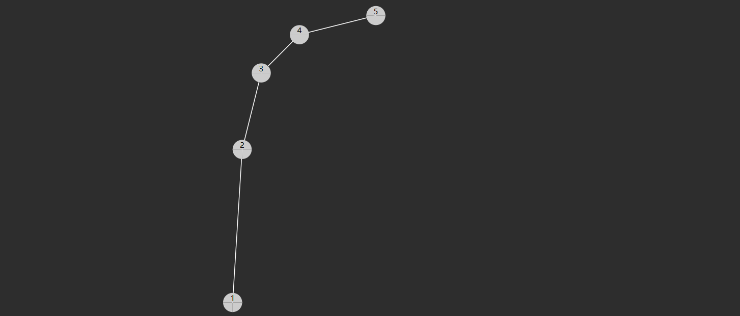
左左型（LL）

• 失衡节点（图中节点8）的 bf > 1，即左边更高
• 失衡节点的左孩子（图中节点6）的 bf >= 0 即左孩子这边也是左边更高或等高

左右型（LR）

• 失衡节点（图中节点8）的 bf > 1，即左边更高
• 失衡节点的左孩子（图中节点3）的 bf < 0 即左孩子这边是右边更高

右左型（RL）

• 失衡节点（图中节点3）的 bf <-1，即右边更高，
• 失衡节点的右孩子（图中节点6）的 bf > 0，即右孩子这边左边更高。

右右型（RR）

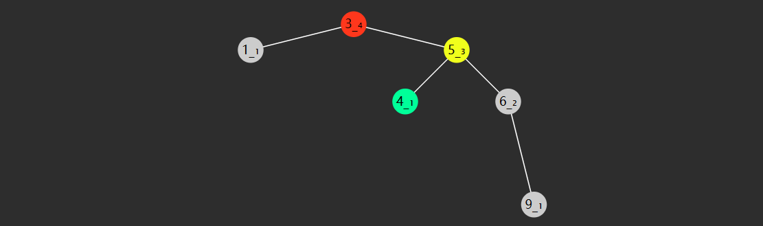
• 失衡节点（图中节点3）的 bf <-1，即右边更高
• 失衡节点的右孩子（图中节点6）的 bf <= 0，即右孩子这边右边更高或等高

解决失衡

失衡可以通过树的旋转解决。什么是树的旋转呢？它是在不干扰元素顺序的情况下更改结构，通常用来让树的高度变得平衡。

观察下面一棵二叉搜索树，可以看到，旋转后，并未改变树的左小右大特性，但根、父、孩子节点都发生了变化。

      4                                   2
     / \             4 right             / \
    2   5      -------------------->    1   4
   / \         <--------------------       / \
  1   3              2 left               3   5

右旋（处理LL型失衡）

旋转前

• 红色节点，旧根（失衡节点）
• 黄色节点，旧根的左孩子，将来作为新根，旧根是它右孩子
• 绿色节点，新根的右孩子，将来要托孤作为旧根的左孩子

旋转后

代码

private AVLNode rightRotate(AVLNode red) {
    AVLNode yellow = red.left;
    AVLNode green = yellow.right;
    yellow.right = red;
    red.left = green;
    return yellow;
}

左旋（处理RR型失衡）

旋转前

• 红色节点，旧根（失衡节点）
• 黄色节点，旧根的右孩子，将来作为新根，旧根是它左孩子
• 绿色节点，新根的左孩子，将来要换托孤作为旧根的右孩子

旋转后

代码

private AVLNode leftRotate(AVLNode red) {
    AVLNode yellow = red.right;
    AVLNode green = yellow.left;
    yellow.left = red;
    red.right = green;
    return yellow;
}

左右旋（处理LR型失衡）

指先左旋左子树，再右旋根节点（失衡节点），这时一次旋转并不能解决失衡（其实就是把LR型失衡先转换成LL型失衡再处理）。

左子树旋转前

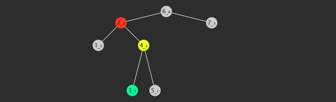
左子树旋转后

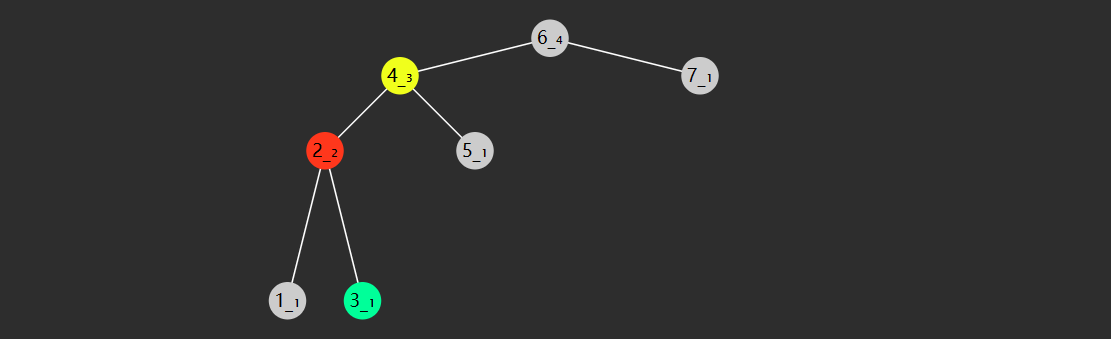
根右旋前

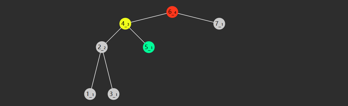
根右旋后

代码

private AVLNode leftRightRotate(AVLNode root) {
    root.left = leftRotate(root.left);
    return rightRotate(root);
}

右左旋（处理RL型失衡）

指先右旋右子树，再左旋根节点（失衡节点）（其实就是把RL型失衡先转换成RR型失衡再处理）。

右子树右旋前

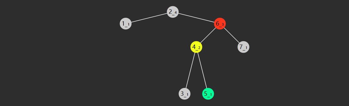
右子树右旋后

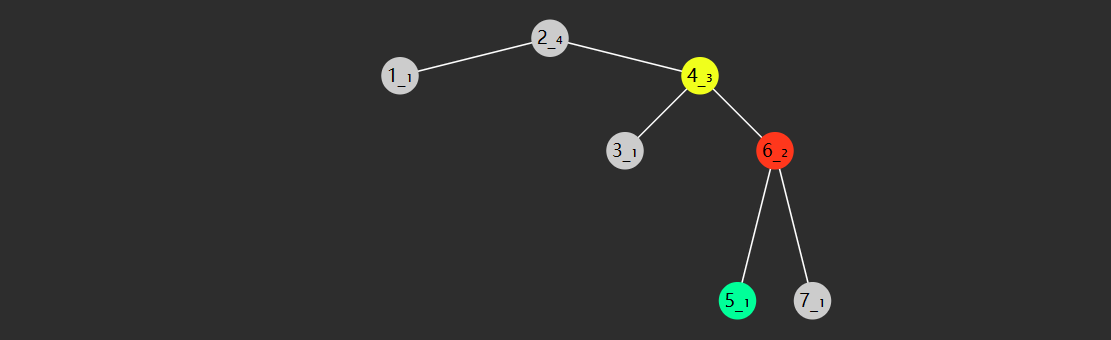
根左旋前

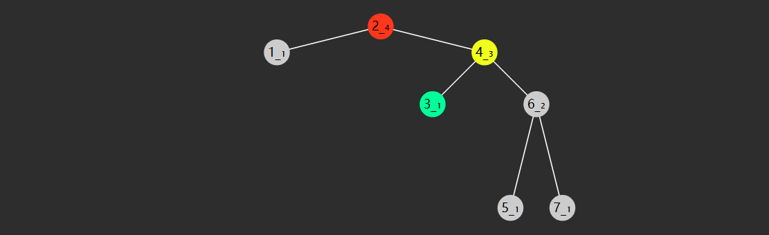
根左旋后

代码

private AVLNode rightLeftRotate(AVLNode root) {
    root.right = rightRotate(root.right);
    return leftRotate(root);
}

注意

每次旋转后，都需要更新高度，需要更新的节点是红色、黄色，而绿色节点高度不变。

仔细观察可以发现，每次旋转时，以红色和黄色节点为根节点的二叉树结构都会发生变化。由于二叉树的节点高度是通过取左右子树中较大高度加1来计算得出的，因此每次旋转后，红色和黄色节点的高度都需要进行更新。

例如，在右旋的例子中，红色节点4的左子树由黄色节点2变为绿色节点3，而黄色节点2的右子树则由绿色节点3变为红色节点4，其余节点的结构保持不变。

旋转前

旋转后

在右旋、左旋中加入更新高度的代码

右旋

private AVLNode rightRotate(AVLNode red) {
    AVLNode yellow = red.left;
    AVLNode green = yellow.right;
    yellow.right = red;
    red.left = green;
    updateHeight(red);
    updateHeight(yellow);
    return yellow;
}

左旋

private AVLNode leftRotate(AVLNode red) {
    AVLNode yellow = red.right;
    AVLNode green = yellow.left;
    yellow.left = red;
    red.right = green;
    updateHeight(red);
    updateHeight(yellow);
    return yellow;
}

这里也有一个需要注意的点，更新高度时我们要从下往上更新，也就是先更新红色节点，再更新黄色节点。

判断及调整平衡代码

private AVLNode balance(AVLNode node) {
    if (node == null) {
        return null;
    }
    int bf = bf(node);
    if (bf > 1 && bf(node.left) >= 0) { //LL型
        return rightRotate(node);
    } else if (bf > 1 && bf(node.left) < 0) { //LR型
        return leftRightRotate(node);
    } else if (bf < -1 && bf(node.right) > 0) { //RL型
        return rightLeftRotate(node);
    } else if (bf < -1 && bf(node.right) <= 0) { //RR型
        return rightRotate(node);
    }
    return node;
}

代码实现

AVL树的实现与二叉搜索树相似，主要区别在于新增和删除操作时需要进行平衡调整。

新增

public void put(int key, Object val) {
    root = doPut(root, key, val);
}

private AVLNode doPut(AVLNode node, int key, Object val) {
    if (node == null) {
        return new AVLNode(key,val);
    }
    if (key == node.key) {
        node.val = val;
        return node;
    }
    if (key < node.key) {
        node.left = doPut(node.left, key, val);
    }
    if (key > node.key) {
        node.right = doPut(node.right, key, val);
    }
    updateHeight(node);
    return balance(node);
}

删除

public void remove(int key) {
    root = doRemove(root, key);
}

private AVLNode doRemove(AVLNode node, int key) {
    if (node == null) {
        return null;
    }

    if (key < node.key) {
        node.left = doRemove(node.left, key);
    }

    if (key > node.key) {
        node.right = doRemove(node.right, key);
    }

    if (key == node.key) {
        if (node.left == null) {
            node = node.right;
        } else if (node.right == null) {
            node = node.left;
        } else {
            AVLNode replaced = node.right;
            while (replaced.left != null) {
                replaced = replaced.left;
            }
            replaced.right = doRemove(node, replaced.key);
            replaced.left = node.left;
            node = replaced;
        }
    }
    updateHeight(node);
    return balance(node);
}

完整代码

public class AVLTree {

    AVLNode root;

    static class AVLNode {
        int key;
        Object value;
        AVLNode left;
        AVLNode right;
        int height = 1; 

        public AVLNode(int key, Object value) {
            this.key = key;
            this.value = value;
        }

        public AVLNode(int key) {
            this.key = key;
        }

        public AVLNode(int key, Object value, AVLNode left, AVLNode right) {
            this.key = key;
            this.value = value;
            this.left = left;
            this.right = right;
        }
    }

    private int height(AVLNode node) {
        return node == null ? 0 : node.height;
    }

    private void updateHeight(AVLNode node) {
        node.height = Integer.max(height(node.left), height(node.right)) + 1;
    }

    private int bf(AVLNode node) {
        return height(node.left) - height(node.right);
    }

    private AVLNode rightRotate(AVLNode red) {
        AVLNode yellow = red.left;
        AVLNode green = yellow.right;
        yellow.right = red;   
        red.left = green;     
        updateHeight(red);
        updateHeight(yellow);
        return yellow;
    }

    private AVLNode leftRotate(AVLNode red) {
        AVLNode yellow = red.right;
        AVLNode green = yellow.left;
        yellow.left = red;
        red.right = green;
        updateHeight(red);
        updateHeight(yellow);
        return yellow;
    }

    private AVLNode leftRightRotate(AVLNode node) {
        node.left = leftRotate(node.left);
        return rightRotate(node);
    }

    private AVLNode rightLeftRotate(AVLNode node) {
        node.right = rightRotate(node.right);
        return leftRotate(node);
    }

    private AVLNode balance(AVLNode node) {
        if (node == null) {
            return null;
        }
        int bf = bf(node);
        if (bf > 1 && bf(node.left) >= 0) { // LL
            return rightRotate(node);
        } else if (bf > 1 && bf(node.left) < 0) { // LR
            return leftRightRotate(node);
        } else if (bf < -1 && bf(node.right) > 0) { // RL
            return rightLeftRotate(node);
        } else if (bf < -1 && bf(node.right) <= 0) { // RR
            return leftRotate(node);
        }
        return node;
    }

    public void put(int key, Object value) {
        root = doPut(root, key, value);
    }

    private AVLNode doPut(AVLNode node, int key, Object value) {
        if (node == null) {
            return new AVLNode(key, value);
        }
        
        if (key == node.key) {
            node.value = value;
            return node;
        }
        
        if (key < node.key) {
            node.left = doPut(node.left, key, value); 
        } else {
            node.right = doPut(node.right, key, value); 
        }
        updateHeight(node);
        return balance(node);
    }

    public void remove(int key) {
        root = doRemove(root, key);
    }

    private AVLNode doRemove(AVLNode node, int key) {
        if (node == null) {
            return null;
        }

        if (key < node.key) {
            node.left = doRemove(node.left, key);
        } else if (node.key < key) {
            node.right = doRemove(node.right, key);
        } else {
            if (node.left == null && node.right == null) {
                return null;
            } else if (node.left == null) {
                node = node.right;
            } else if (node.right == null) {
                node = node.left;
            } else {
                AVLNode s = node.right;
                while (s.left != null) {
                    s = s.left;
                }

                s.right = doRemove(node.right, s.key);
                s.left = node.left;
                node = s;
            }
        }

        updateHeight(node);

        return balance(node);
    }
}

总结

AVL树是一种自平衡二叉搜索树，通过对每个节点的左右子树高度差进行控制，保持树的平衡，确保查找、插入和删除操作的时间复杂度始终为O(log n)。由于树的高度受到严格限制，因此在节点数目较多且查找操作频繁的情况下，AVL树能够提供高效的查找性能。每次插入或删除节点时，AVL树会通过旋转操作来保持平衡，这确保了树的深度不会过大，从而避免了退化成链表的情况。

然而，AVL树的插入和删除操作较为复杂，每次修改树结构时都可能需要进行旋转操作，增加了实现的复杂度和时间开销。特别是在频繁进行插入和删除操作时，旋转操作可能成为性能瓶颈。因此，在节点较少或插入、删除操作占比较高的场景中，AVL树的性能优势可能不如其他数据结构，如红黑树。红黑树虽然也能保持平衡，但其旋转操作较少，适用于插入和删除较为频繁的情况，因此在这些应用场景下更为高效。

红黑树

红黑树是一种自平衡二叉查找树，最早由一位名叫鲁道夫·贝尔的德国计算机科学家于1972年发明。然而，最初的树形结构不是现在的红黑树，而是一种称为B树的结构，它是一种多叉树，可用于在磁盘上存储大量数据。

在1980年代早期，计算机科学家利奥尼达斯·J·吉巴斯和罗伯特·塞奇威克推广了红黑树，并证明了它的自平衡性和高效性。从那时起，红黑树成为了最流行的自平衡二叉查找树之一，并被广泛应用于许多领域，如编译器、操作系统、数据库等。

红黑树的名字来源于红色节点和黑色节点的交替出现，它们的颜色是用来维护树的平衡性的关键。它们的颜色具有特殊的意义，黑色节点代表普通节点，而红色节点代表一个新添加的节点，它们必须满足一些特定的规则才能维持树的平衡性。

概述

红黑树也是一种自平衡的二叉搜索树，较之 AVL，插入和删除时旋转次数更少。

红黑树特性

1. 所有节点都有两种颜色：红🔴、黑⚫
2. 每个叶子节点（null节点）都视为黑色⚫
3. 红色🔴节点不能相邻
4. 根节点是黑色⚫
5. 从根节点到任意一个叶子节点，路径中的黑色⚫节点数一样（黑色完美平衡）

根据上面的性质，判断一下下面这棵树是不是红黑树

先下结论，这棵树不是红黑树。

上面这棵树首先很容易就能看出是满足特性1-4条的，关键在于第5条特性，可能乍一看好像也是符合第5条的，但实际就会陷入一个误区，忽略了null节点，这样看的话每一条从根节点到叶子结点的路径确实都经过了两个黑色节点。

但实际上，在红黑树中，最下面的null节点也是需要考虑到的，如下图

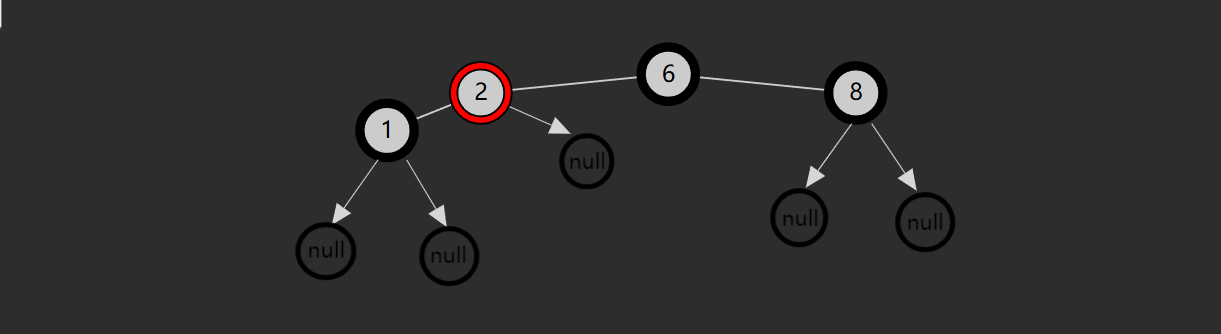
这样一来，每一条从根节点到叶子结点的路径经过的黑色节点数量也不是全都一样，这样特性5就不满足了，所以这棵树并不是一棵红黑树。

推论

1. 红黑树的子树也一定是红黑树。
2. 根节点以外如果所有节点都有兄弟，那么可以不用考虑null节点
3. 在没有考虑null节点的情况下，根节点以外如果某个节点没有兄弟且包含黑色节点，肯定违反了红黑树特性5
4. 根据推论2和特性3，可以推出，根节点以外如果某个节点没有兄弟，那他必定是红色节点，且它的两个孩子必定为null
5. 根据推论2和特性3，还可以推出，一个红色节点，他只能是有两个黑孩子或者两个孩子都为null

准备工作

枚举类

enum Color {
    RED, BLACK;
}

红黑树的颜色有两种，红色和黑色，所以这里先定义一个枚举类型，用来代表两种颜色。

节点类

static class Node {
    int key;
    Object value;
    Node left;
    Node right;
    Node parent;        //父节点 操作红黑树时，需要维护parent指向正确的对象
    Color color = RED;  //颜色 默认为红色
    
	// ...
	
    // 是否是左孩子
    boolean isLeftChild() {
        return parent != null && parent.left == this; //节点是根节点时父亲为null
    }

    // 叔叔
    Node uncle() {
        if (parent == null || parent.parent == null) { //节点是根节点或者节点的父节点是根节点都是没有叔叔节点的
            return null;
        }
        if (parent.isLeftChild()) {
            return parent.parent.right;
        } else {
            return parent.parent.left;
        }
    }

    // 兄弟
    Node sibling() {
        if (parent == null) { // 根节点没有兄弟节点
            return null;
        }
        if (this.isLeftChild()) {
            return parent.right;
        } else {
            return parent.left;
        }
    }
}

两个比较特殊的属性：parent（父节点）和color（颜色），三个工具方法：isLeftChild（是否是左孩子）、uncle（获取叔叔节点）、sibling（获取兄弟节点）。后面操作红黑树时，这些东西会经常用到，先定义出来，能让我们后面的代码更简洁，思路也更清晰。

根据特性1，红黑树节点的颜色要么是红色要么是黑色，那么在插入新节点时，这个节点应该是红色还是黑色呢？答案是红色，原因也不难理解。如果插入的节点是黑色，那么这个节点所在路径比其他路径多出一个黑色节点，这个调整起来会比较麻烦。如果插入的节点是红色，此时所有路径上的黑色节点数量不变，仅可能会出现红红相邻的情况，违反了特性4，这种情况下，调整起来相对简单，通过变色和旋转进行调整即可。

判断红、黑

// 判断红
boolean isRed(Node node) {
	return node != null && node.color == RED;
}

// 判断黑
boolean isBlack(Node node) {
	return !isRed(node);
}

方便处理节点为null的情况

右旋、左旋

// 右旋
private void rightRotate(Node pink) {
    Node parent = pink.parent;
    Node yellow = pink.left;
    Node green = yellow.right;
    if (green != null) {
        green.parent = pink;
    }
    yellow.right = pink;
    yellow.parent = parent;
    pink.left = green;
    pink.parent = yellow;
    //建立新根yellow与parent的父子关系
    if (parent == null) {
        root = yellow;
    } else if (parent.left == pink) {
        parent.left = yellow;
    } else {
        parent.right = yellow;
    }
}

// 左旋
private void leftRotate(Node pink) {
    Node parent = pink.parent;
    Node yellow = pink.right;
    Node green = yellow.left;
    if (green != null) {
        green.parent = pink;
    }
    yellow.left = pink;
    yellow.parent = parent;
    pink.right = green;
    pink.parent = yellow;
    //建立新根yellow与parent的父子关系
    if (parent == null) {
        root = yellow;
    } else if (parent.left == pink) {
        parent.left = yellow;
    } else {
        parent.right = yellow;
    }
}

两个需要注意的点：

• 维护各节点的parent指向正确的对象
• 旋转后新根与父节点的父子关系在方法内直接建立

红黑树的操作

红黑树的基本操作和其他树形结构一样，一般都包括查找、插入、删除等操作。前面说到，红黑树是一种自平衡的二叉查找树，既然是二叉查找树的一种，那么查找过程和二叉查找树一样，比较简单，这里不再赘述。相对于查找操作，红黑树的插入和删除操作就要复杂的多。尤其是删除操作，要处理的情况比较多，下面就来分情况讲解。

插入和删除时的各种情况的例子

不过仔细观察可以发现，操作红黑树后，只有两种情况下红黑树需要重新调整平衡

• 红红相连
• 黑色不平衡

插入

前面讲过，插入节点默认为红色。

case 1：插入节点为根节点，将根节点变黑⚫

case 2：插入节点的父亲为黑色⚫，树的红黑性质不变，无需调整

插入节点的父亲为红色🔴，触发红红相邻

case 3：叔叔为红色🔴

• 父亲变为黑色⚫，为了保证黑色平衡，连带的叔叔也变为黑色⚫
• 祖父如果是黑色不变，会造成这颗子树黑色过多，因此祖父节点变为红色🔴
• 祖父如果变成红色，可能会接着触发红红相邻，因此对将祖父进行递归调整
• 往上递归会一直持续，直到出现以下三种结果：
  • 祖父的父亲是黑色，没有触发红红相邻，进入case2，结束递归
  • 递归到根节点的孩子节点，根据特性4，根节点一定是黑色，因此会进入case2，结束递归
  • 递归到根节点，进入case1，将根节点变成黑色，结束递归，而且经过重复递归调整，整棵红黑树恢复平衡，因为根节点没有兄弟节点，也就不用考虑根节点与兄弟节点的黑色平衡

case 4：叔叔为黑色⚫

• 父亲为左孩子，插入节点也是左孩子，此时即 LL 不平衡

  • 让父亲变黑⚫，为了保证这颗子树黑色不变，将祖父变成红🔴，但叔叔子树少了一个黑色
  • 祖父右旋，补齐一个黑色给叔叔，父亲旋转上去取代祖父，由于它是黑色，不会再次触发红红相邻

• 父亲为左孩子，插入节点是右孩子，此时即 LR 不平衡

  • 父亲左旋，变成 LL 情况，按 LL 不平衡来后续处理

• 父亲为右孩子，插入节点也是右孩子，此时即 RR 不平衡

  • 让父亲变黑⚫，为了保证这颗子树黑色不变，将祖父变成红🔴，但叔叔子树少了一个黑色

  • 祖父左旋，补齐一个黑色给叔叔，父亲旋转上去取代祖父，由于它是黑色，不会再次触发红红相邻

• 父亲为右孩子，插入节点是左孩子，此时即 RL 不平衡

  • 父亲右旋，变成 RR 情况，按 RR 不平衡来后续处理

public void put(int key, Object value) {
    Node p = root;
    Node parent = null;
    while (p != null) {
        parent = p;
        if (key < p.key) {
            p = p.left;
        } else if (p.key < key) {
            p = p.right;
        } else {
            p.value = value; // 更新
            return;
        }
    }
    Node inserted = new Node(key, value);
    if (parent == null) {
        root = inserted;
    } else if (key < parent.key) {
        parent.left = inserted;
        inserted.parent = parent;
    } else {
        parent.right = inserted;
        inserted.parent = parent;
    }
    fixRedRed(inserted);
}


void fixRedRed(Node x) {
    // case 1 插入节点是根节点，变黑即可
    if (x == root) {
        x.color = BLACK;
        return;
    }
    // case 2 插入节点父亲是黑色，无需调整
    if (isBlack(x.parent)) {
        return;
    }
    /* case 3 当红红相邻，叔叔为红时
        需要将父亲、叔叔变黑、祖父变红，然后对祖父做递归处理
    */
    Node parent = x.parent;
    Node uncle = x.uncle();
    Node grandparent = parent.parent;
    if (isRed(uncle)) {
        parent.color = BLACK;
        uncle.color = BLACK;
        grandparent.color = RED;
        fixRedRed(grandparent);
        return;
    }

    // case 4 当红红相邻，叔叔为黑时
    if (parent.isLeftChild() && x.isLeftChild()) { // LL
        parent.color = BLACK;
        grandparent.color = RED;
        rightRotate(grandparent);
    } else if (parent.isLeftChild() && !x.isLeftChild()) { // LR
        leftRotate(parent);
        x.color = BLACK;
        grandparent.color = RED;
        rightRotate(grandparent);
    } else if (!parent.isLeftChild() && !x.isLeftChild()) { // RR
        parent.color = BLACK;
        grandparent.color = RED;
        leftRotate(grandparent);
    } else { // RL
        rightRotate(parent);
        x.color = BLACK;
        grandparent.color = RED;
        leftRotate(grandparent);
    }
}

删除

case0：删除节点有两个孩子

• 交换删除节点和后继节点的 key，value，递归删除后继节点，后继节点必定最多只有一个右孩子，所以会直接进入以下其他case

删除节点没有孩子或只剩一个孩子

case 1：删的是根节点

• 根节点没有孩子，删完了，直接将 root = null
• 根节点只剩一个孩子，用剩余节点替换了根节点的 key，value，根节点孩子 = null，颜色保持黑色⚫不变

如果删除的节点是红色直接删除，不用作任何调整。但删黑色有一种简单情况

case 2：删的是黑⚫，替换节点是红🔴

• 让这个替换的红节点变黑⚫，补上删除失去的黑色资源

替换节点是黑色⚫，触发双黑（本质上是少了一个黑），删除节点和替换节点都是黑色⚫，所以没法通过将替换节点变成黑色来补上删除节点失去的黑色资源。

注意！！！删除节点只剩一个孩子节点的情况下，是不会触发双黑的，因为在这个情况下，替换节点只能是删除节点剩下的那个孩子节点，但是红黑树不会存在一个黑色节点没有兄弟节点的情况。

如何让黑色资源重新平衡？可以借助兄弟的力量，于是有了这几种情况

case 3：删除节点的兄弟节点为红🔴

• 过度情况，可通过旋转变成case 4或者case 5
• 兄弟节点为红，父节点、侄子节点必定是黑，要不就触发红红相邻了
• 而且侄子节点必定不为null，要不黑色平衡不了
• 删除节点是左孩子节点，父节点左旋
• 删除节点是右孩子节点，父节点右旋
• 父节点和兄弟节点要变色，保证旋转后颜色平衡
• 旋转的目的是让黑侄子节点变为删除节点的黑兄弟节点，对删除节点再次递归，进入 case 4 或 case 5

case 4：删除节点的兄弟节点为黑色⚫，两个侄子节点都为黑 ⚫

• 将兄弟节点变红🔴，目的是将删除节点和兄弟节点那边的黑色数目同时减 1，先达成两兄弟之间的内部黑色平衡
• 如果父节点是红🔴，则需将父节点变为黑，避免红红，且此时路径黑节点数目刚好与删除节点前保持一致
• 如果父节点是黑⚫，说明这条路径还是少黑，再次让父节点触发双黑，进入递归
• 如果一直递归到根节点，所有路径都会比原来少一个黑色，红黑树又恢复平衡，结束递归

case 5：删除节点的兄弟节点为黑⚫，至少一个红🔴侄子

• 如果兄弟节点是左孩子节点，左侄子节点是红🔴，LL 不平衡

  • 父节点右旋
  • 将来删除节点这边少个黑，所以最后旋转过来的父节点需要变成黑⚫，平衡起见，左侄子节点也变黑⚫
  • 原来兄弟节点要成为新的父节点，需要变成原来父节点颜色

• 如果兄弟节点是左孩子节点，右侄子节点是红🔴，LR 不平衡

  • 兄弟节点左旋，然后父节点右旋
  • 将来删除节点这边少个黑，所以最后旋转过来的父节点需要变成黑⚫
  • 原来右侄子节点要成为新的父节点，需要变成原来父节点颜色
  • 兄弟节点已经是黑了⚫，无需改变

• 如果兄弟节点是右孩子节点，右侄子节点是红🔴，RR 不平衡

  • 父节点左旋
  • 将来删除节点这边少个黑，所以最后旋转过来的父节点需要变成黑⚫，平衡起见，右侄子节点也变黑⚫
  • 原来兄弟节点要成为新的父节点，需要变成原来父节点颜色

• 如果兄弟节点是右孩子节点，左侄子节点是红🔴，RL 不平衡

  • 兄弟节点右旋，然后父节点左旋
  • 将来删除节点这边少个黑，所以最后旋转过来的父节点需要变成黑⚫
  • 原来左侄子节点要成为新的父节点，需要变成原来父节点颜色
  • 兄弟节点已经是黑了⚫，无需改变

我们将父节点，兄弟节点，删除节点看成一个待调整区域，可以发现，case 5 看似复杂，其实四个情况都是做同一件事，将红侄子节点通过旋转拉进待调整区域，通过将红侄子变成黑色补上删除节点失去的一个黑色节点，且不改变待调整区域各位置的节点颜色，所以旋转后都要调整颜色，将待调整区域各个位置的节点颜色恢复成原来的颜色。

这里讲的有点抽象，我们通过画图观察，这样会更具体一点

其实待调整区域这里只会出现两种情况

      红         			  红									 黑         			  黑
	 / \     ---------->     / \									 / \     ---------->     / \
    黑  黑      调整完       黑  黑								   黑  黑       调整完       黑  黑

当然，调整前后也并不是完全一样，侄子节点会顶替删除节点进入待调整区域内，当然，侄子节点不是出现在删除节点的位置上

例如，在LL的情况里

调整前

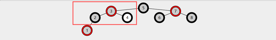
调整后

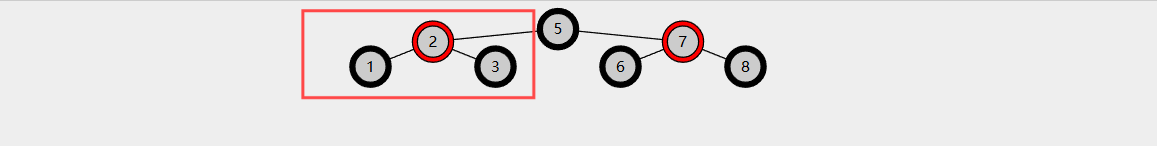
其中，4是删除节点，3是父亲节点，2是兄弟节点，1是侄子节点

为什么这样做就可以让红黑树恢复平衡？我们将待调整区域以外的区域看成外部区域，可以发现，只要父节点不改变颜色并且以父节点内部各路径黑色数目与原来保持一致（问题A)，那么外部区域不需要任何调整，整棵红黑树也会恢复平衡。

如何解决问题A，核心思路就是让待调整区域里不失去任何一个位置的节点并且各位置的节点颜色与原来保持一致，但是我们的删除节点就在待调整区域里，我们也不能因为解决问题A而让其他区域的黑色数目减少，这怎么办？不要忘了我们还有一个红色侄子节点，我们可以通过旋转把它拉近待调整区域，再通过调整颜色将待调整区域各个位置的节点颜色恢复成原来的颜色，这样做会导致外部区域丢失一个红色节点，但是，红节点的丢失是不会对红黑树的平衡造成影响的。

public void remove(int key) {
    Node deleted = find(key);
    if (deleted == null) {
        return;
    }
    doRemove(deleted);
}

public boolean contains(int key) {
    return find(key) != null;
}

// 查找删除节点
private Node find(int key) {
    Node p = root;
    while (p != null) {
        if (key < p.key) {
            p = p.left;
        } else if (p.key < key) {
            p = p.right;
        } else {
            return p;
        }
    }
    return null;
}

// 查找剩余节点
private Node findReplaced(Node deleted) {
    if (deleted.left == null && deleted.right == null) {
        return null;
    }
    if (deleted.left == null) {
        return deleted.right;
    }
    if (deleted.right == null) {
        return deleted.left;
    }
    Node s = deleted.right;
    while (s.left != null) {
        s = s.left;
    }
    return s;
}

// 处理双黑 (case3、case4、case5) (删除的节点是黑色，替换上来的节点也是黑色)
private void fixDoubleBlack(Node x) {
    if (x == root) {
        return;
    }
    Node parent = x.parent;
    Node sibling = x.sibling();
    // case 3 兄弟节点是红色
    if (isRed(sibling)) {
        if (x.isLeftChild()) {
            leftRotate(parent);
        } else {
            rightRotate(parent);
        }
        parent.color = RED;
        sibling.color = BLACK;
        fixDoubleBlack(x);
        return;
    }

    // case 4 兄弟是黑色, 两个侄子也是黑色
    if (isBlack(sibling.left) && isBlack(sibling.right)) {
        sibling.color = RED;
        if (isRed(parent)) {
            parent.color = BLACK;
        } else {
            fixDoubleBlack(parent);
        }
    }
    // case 5 兄弟是黑色, 侄子有红色
    else {
        // LL
        if (sibling.isLeftChild() && isRed(sibling.left)) {
            rightRotate(parent);
            sibling.left.color = BLACK;
            sibling.color = parent.color;
        }
        // LR
        else if (sibling.isLeftChild() && isRed(sibling.right)) {
            sibling.right.color = parent.color;
            leftRotate(sibling);
            rightRotate(parent);
        }
        // RL
        else if (!sibling.isLeftChild() && isRed(sibling.left)) {
            sibling.left.color = parent.color;
            rightRotate(sibling);
            leftRotate(parent);
        }
        // RR
        else {
            leftRotate(parent);
            sibling.right.color = BLACK;
            sibling.color = parent.color;
        }
        parent.color = BLACK;
    }
}

private void doRemove(Node deleted) {
    Node replaced = findReplaced(deleted);
    Node parent = deleted.parent;
    // 没有孩子
    if (replaced == null) {
        // case 1 删除的是根节点
        if (deleted == root) {
            root = null;
        } else {
            //没有孩子，替换节点是null，根据红黑树特性，null也是黑色，如果删除的也是黑色，其实就已经触发了双黑
            if (isBlack(deleted)) {
                // 复杂调整
                fixDoubleBlack(deleted);
            } else {
                // 红色叶子, 无需任何处理
            }
            if (deleted.isLeftChild()) {
                parent.left = null;
            } else {
                parent.right = null;
            }
            deleted.parent = null;
        }
        return;
    }
    // 有一个孩子
    if (deleted.left == null || deleted.right == null) {
        // case 1 删除的是根节点
        if (deleted == root) {
            root.key = replaced.key;
            root.value = replaced.value;
            root.left = root.right = null;
        } else {
            if (deleted.isLeftChild()) {
                parent.left = replaced;
            } else {
                parent.right = replaced;
            }
            replaced.parent = parent;
            deleted.left = deleted.right = deleted.parent = null;
            // case 2 只有一个孩子的情况下，删除节点必定是黑，替换节点（也就是删除节点唯一一个孩子）必定是红，直接让替换节点变黑补上删除的一个黑色
            replaced.color = BLACK;

        }
        return;
    }
    // case 0 有两个孩子 => 有一个孩子 或 没有孩子
    int t = deleted.key;
    deleted.key = replaced.key;
    replaced.key = t;

    Object v = deleted.value;
    deleted.value = replaced.value;
    replaced.value = v;
    doRemove(replaced);
}

完整代码

public class RedBlackTree {

    enum Color {
        RED, BLACK;
    }

    Node root;

    static class Node {
        int key;
        Object value;
        Node left;
        Node right;
        Node parent;
        Color color = RED;

        public Node(int key, Object value) {
            this.key = key;
            this.value = value;
        }

        public Node(int key) {
            this.key = key;
        }

        public Node(int key, Color color) {
            this.key = key;
            this.color = color;
        }

        public Node(int key, Color color, Node left, Node right) {
            this.key = key;
            this.color = color;
            this.left = left;
            this.right = right;
            if (left != null) {
                left.parent = this;
            }
            if (right != null) {
                right.parent = this;
            }
        }

        boolean isLeftChild() {
            return parent != null && parent.left == this;
        }

        Node uncle() {
            if (parent == null || parent.parent == null) {
                return null;
            }
            if (parent.isLeftChild()) {
                return parent.parent.right;
            } else {
                return parent.parent.left;
            }
        }

        Node sibling() {
            if (parent == null) {
                return null;
            }
            if (this.isLeftChild()) {
                return parent.right;
            } else {
                return parent.left;
            }
        }
    }

    boolean isRed(Node node) {
        return node != null && node.color == RED;
    }

    boolean isBlack(Node node) {
//        return !isRed(node);
        return node == null || node.color == BLACK;
    }

    private void rightRotate(Node pink) {
        Node parent = pink.parent;
        Node yellow = pink.left;
        Node green = yellow.right;
        if (green != null) {
            green.parent = pink;
        }
        yellow.right = pink;
        yellow.parent = parent;
        pink.left = green;
        pink.parent = yellow;
        if (parent == null) {
            root = yellow;
        } else if (parent.left == pink) {
            parent.left = yellow;
        } else {
            parent.right = yellow;
        }
    }

    private void leftRotate(Node pink) {
        Node parent = pink.parent;
        Node yellow = pink.right;
        Node green = yellow.left;
        if (green != null) {
            green.parent = pink;
        }
        yellow.left = pink;
        yellow.parent = parent;
        pink.right = green;
        pink.parent = yellow;
        if (parent == null) {
            root = yellow;
        } else if (parent.left == pink) {
            parent.left = yellow;
        } else {
            parent.right = yellow;
        }
    }
 
    public void put(int key, Object value) {
        Node p = root;
        Node parent = null;
        while (p != null) {
            parent = p;
            if (key < p.key) {
                p = p.left;
            } else if (p.key < key) {
                p = p.right;
            } else {
                p.value = value;
                return;
            }
        }
        Node inserted = new Node(key, value);
        if (parent == null) {
            root = inserted;
        } else if (key < parent.key) {
            parent.left = inserted;
            inserted.parent = parent;
        } else {
            parent.right = inserted;
            inserted.parent = parent;
        }
        fixRedRed(inserted);
    }

    void fixRedRed(Node x) {
        if (x == root) {
            x.color = BLACK;
            return;
        }
        if (isBlack(x.parent)) {
            return;
        }
       
        Node parent = x.parent;
        Node uncle = x.uncle();
        Node grandparent = parent.parent;
        if (isRed(uncle)) {
            parent.color = BLACK;
            uncle.color = BLACK;
            grandparent.color = RED;
            fixRedRed(grandparent);
            return;
        }

        if (parent.isLeftChild() && x.isLeftChild()) { // LL
            parent.color = BLACK;
            grandparent.color = RED;
            rightRotate(grandparent);
        } else if (parent.isLeftChild()) { // LR
            leftRotate(parent);
            x.color = BLACK;
            grandparent.color = RED;
            rightRotate(grandparent);
        } else if (!x.isLeftChild()) { // RR
            parent.color = BLACK;
            grandparent.color = RED;
            leftRotate(grandparent);
        } else { // RL
            rightRotate(parent);
            x.color = BLACK;
            grandparent.color = RED;
            leftRotate(grandparent);
        }
    }

    public void remove(int key) {
        Node deleted = find(key);
        if (deleted == null) {
            return;
        }
        doRemove(deleted);
    }

    public boolean contains(int key) {
        return find(key) != null;
    }

    private Node find(int key) {
        Node p = root;
        while (p != null) {
            if (key < p.key) {
                p = p.left;
            } else if (p.key < key) {
                p = p.right;
            } else {
                return p;
            }
        }
        return null;
    }

    private Node findReplaced(Node deleted) {
        if (deleted.left == null && deleted.right == null) {
            return null;
        }
        if (deleted.left == null) {
            return deleted.right;
        }
        if (deleted.right == null) {
            return deleted.left;
        }
        Node s = deleted.right;
        while (s.left != null) {
            s = s.left;
        }
        return s;
    }

    private void fixDoubleBlack(Node x) {
        if (x == root) {
            return;
        }
        Node parent = x.parent;
        Node sibling = x.sibling();
        if (isRed(sibling)) {
            if (x.isLeftChild()) {
                leftRotate(parent);
            } else {
                rightRotate(parent);
            }
            parent.color = RED;
            sibling.color = BLACK;
            fixDoubleBlack(x);
            return;
        }
        if (sibling != null) {
            if (isBlack(sibling.left) && isBlack(sibling.right)) {
                sibling.color = RED;
                if (isRed(parent)) {
                    parent.color = BLACK;
                } else {
                    fixDoubleBlack(parent);
                }
            }
            else {
                if (sibling.isLeftChild() && isRed(sibling.left)) {
                    rightRotate(parent);
                    sibling.left.color = BLACK;
                    sibling.color = parent.color;
                }
                else if (sibling.isLeftChild() && isRed(sibling.right)) {
                    sibling.right.color = parent.color;
                    leftRotate(sibling);
                    rightRotate(parent);
                }
                else if (!sibling.isLeftChild() && isRed(sibling.left)) {
                    sibling.left.color = parent.color;
                    rightRotate(sibling);
                    leftRotate(parent);
                }
                else {
                    leftRotate(parent);
                    sibling.right.color = BLACK;
                    sibling.color = parent.color;
                }
                parent.color = BLACK;
            }
        } else {
            fixDoubleBlack(parent); // 实际上不会出现这种情况
        }
    }

    private void doRemove(Node deleted) {
        Node replaced = findReplaced(deleted);
        Node parent = deleted.parent;
        if (replaced == null) {
            if (deleted == root) {
                root = null;
            } else {
                if (isBlack(deleted)) {
                    fixDoubleBlack(deleted);
                } else {
                    // 删除节点是红色，不用做平衡调整
                }
                if (deleted.isLeftChild()) {
                    parent.left = null;
                } else {
                    parent.right = null;
                }
                deleted.parent = null;
            }
            return;
        }
        if (deleted.left == null || deleted.right == null) {
            if (deleted == root) {
                root.key = replaced.key;
                root.value = replaced.value;
                root.left = root.right = null;
            } else {
                if (deleted.isLeftChild()) {
                    parent.left = replaced;
                } else {
                    parent.right = replaced;
                }
                replaced.parent = parent;
                deleted.left = deleted.right = deleted.parent = null;
                if (isBlack(deleted) && isBlack(replaced)) { // 实际上不会出现这种情况
                    fixDoubleBlack(replaced);
                } else {
                    replaced.color = BLACK;
                }
            }
            return;
        }
        
        int t = deleted.key;
        deleted.key = replaced.key;
        replaced.key = t;

        Object v = deleted.value;
        deleted.value = replaced.value;
        replaced.value = v;
        doRemove(replaced);
    }
}

总结

维度	普通二叉搜索树	AVL树	红黑树
查询	平均O(logn)，最坏O(n)	O(logn)	O(logn)
插入	平均O(logn)，最坏O(n)	O(logn)	O(logn)
删除	平均O(logn)，最坏O(n)	O(logn)	O(logn)
平衡性	不平衡	严格平衡	近似平衡
结构	二叉树	自平衡的二叉树	具有红黑性质的自平衡二叉树
查找效率	低	高	高
插入删除效率	低	中等	高

普通二叉搜索树插入、删除、查询的时间复杂度与树的高度相关，因此在最坏情况下，时间复杂度为O(n)，而且容易退化成链表，查找效率低。

AVL树是一种高度平衡的二叉搜索树，其左右子树的高度差不超过1。因此，它能够在logn的平均时间内完成插入、删除、查询操作，但是在维护平衡的过程中，需要频繁地进行旋转操作，导致插入删除效率较低。

红黑树是一种近似平衡的二叉搜索树，它在保持高度平衡的同时，又能够保持较高的插入删除效率。红黑树通过节点着色和旋转操作来维护平衡。红黑树在维护平衡的过程中，能够进行较少的节点旋转操作，因此插入删除效率较高，并且查询效率也较高。

综上所述，红黑树具有较高的综合性能，是一种广泛应用的数据结构。

B树

B树（B-Tree）结构是一种高效存储和查询数据的方法，它的历史可以追溯到1970年代早期。B树的发明人Rudolf Bayer和Edward M. McCreight分别发表了一篇论文介绍了B树。这篇论文是1972年发表于《ACM Transactions on Database Systems》中的，题目为"Organization and Maintenance of Large Ordered Indexes"。

这篇论文提出了一种能够高效地维护大型有序索引的方法，这种方法的主要思想是将每个节点扩展成多个子节点，以减少查找所需的次数。B树结构非常适合应用于磁盘等大型存储器的高效操作，被广泛应用于关系数据库和文件系统中。

B树结构有很多变种和升级版，例如B+树，B*树和SB树等。这些变种和升级版本都基于B树的核心思想，通过调整B树的参数和结构，提高了B树在不同场景下的性能表现。

总的来说，B树结构是一个非常重要的数据结构，为高效存储和查询大量数据提供了可靠的方法。它的历史可以追溯到上个世纪70年代，而且在今天仍然被广泛应用于各种场景。

概述

B的含义

B-树的名称是由其发明者Rudolf Bayer提出的。Bayer和McCreight从未解释B代表什么，人们提出了许多可能的解释，比如Boeing、balanced、between、broad、bushy和Bayer等。但McCreight表示，越是思考B-trees中的B代表什么，就越能更好地理解B-trees

B树的特性

度（degree）指树中节点孩子数

阶（order）指所有节点孩子数的最大值

特性1：节点中 key 可以有多个，以升序存储

特性2：每个非叶子节点中的度数是 key 的数量 + 1、叶子节点度数为 0

特性3：如果根节点不是叶子节点，那么它最少有两个子节点

特性4：最小度数 、key 的数量范围和B树的阶数关系如下：

最小度数 t	key 的数量范围	B树的阶数 m
2	1 ~ 3	4
3	2 ~ 5	6
4	3 ~ 7	8
...	...	...
t	(t - 1) ~ (2t - 1)	2t

其中

• 最小度数至少是2，且除根节点和叶子节点外，其他节点需满足最小度数
• 当节点中 key 的数量达到其最大值时，即 3、5、7 ... 2t - 1，需要分裂
• 除根节点外，当节点中 key 的数量小于其最小值时，即 1、2、3 ... t - 1，需要旋转或合并
• 以最小度数为基准，m = 2t，以阶数为基准，t = ceil(m/2)

特性5：叶子节点的深度都相同

特性6：两个 key（k1，k2）之间的孩子节点的所有 key 都在 (k1，k2) 的范围之内。

例如，图中的 7 和 16 之间的孩子节点 [9, 12] 的所有 key 都满足 7 < key < 16。

问：B-树为什么有最小度数的限制？

答：B树中有最小度数的限制是为了保证B树的平衡特性。

在B树中，每个节点都可以有多个子节点，这使得B树可以存储大量的键值，但也带来了一些问题。如果节点的子节点数量太少，那么就可能导致B树的高度过高，从而降低了B树的效率。此外，如果节点的子节点数量太多，那么就可能导致节点的搜索、插入和删除操作变得复杂和低效。

最小度数的限制通过限制节点的子节点数量，来平衡这些问题。在B树中，每个节点的子节点数量都必须在一定的范围内，即t到2t之间（其中t为最小度数）

B-树与 2-3 树、2-3-4 树的关系

可以这样总结它们之间的关系：

• 2-3树是最小度数为2的B树，其中每个节点可以包含2个或3个子节点。
• 2-3-4树是最小度数为2的B树的一种特殊情况，其中每个节点可以包含2个、3个或4个子节点。
• B树是一种更加一般化的平衡树，可以适应不同的应用场景，其节点可以包含任意数量的键值，节点的度数取决于最小度数t的设定。

实现

节点类

static class Node {
    boolean leaf = true;
    int keyNumber;
    int t;
    int[] keys;
    Node[] children;    

    public Node(int t) {
        this.t = t;
        this.keys = new int[2 * t - 1];
        this.children = new Node[2 * t];
    }
    
}

• leaf 表示是否为叶子节点
• keyNumber 为 keys 中有效 key 数目
• t 为最小度数，它决定了节点中key 的最小、最大数目，分别是 t-1 和 2t-1
• keys 存储此节点的 key
• children 存储此节点的 child

多路查找

为上面节点类添加 get 方法

Node get(int key) {
    int i = 0;
    while (i < keyNumber) {
        if (keys[i] < key) {
            i++;
        } else if (keys[i] > key) {
            break;
        } else {
            return this;
        }        
    }
    // 执行到此时 keys[i]>key 或 i==keyNumber
    if (leaf) {
        return null;
    }
    // 非叶子情况
    return children[i].get(key);
}

插入 key 和 child

为上面节点类添加 insertKey 和 insertChild 方法

void insertKey(int key, int index) {
    System.arraycopy(keys, index, keys, index + 1, keyNumber - index);
    keys[index] = key;
    keyNumber++;
}

void insertChild(Node child, int index) {
    System.arraycopy(children, index, children, index + 1, keyNumber - index);
    children[index] = child;
}

作用是向 keys 数组或 children 数组指定 index 处插入新数据，注意

• 由于使用了静态数组，并且不会在新增或删除时改变它的大小，因此需要额外的 keyNumber 来指定数组内有效 key 的数目
  • 插入时 keyNumber++
  • 删除时减少 keyNumber 的值即可
• children 不会单独维护数目，它比 keys 多一个
• 如果这两个方法同时调用，注意它们的先后顺序，insertChild 后调用，因为它计算复制元素个数时用到了 keyNumber

定义树

public class BTree {
    final int t;
    final int MIN_KEY_NUMBER;
    final int MAX_KEY_NUMBER;
    Node root;

    public BTree() {
        this(2);
    }

    public BTree(int t) {
        this.t = t;
        MIN_KEY_NUMBER = t - 1;
        MAX_KEY_NUMBER = 2 * t - 1;
        root = new Node(t);
    }
    
    public boolean contains(int key) {
        return root.get(key) != null;
    }
}

• t ：树中节点的最小度数
• MIN_KEY_NUMBER：树中节点 key 数量的上限
• MIN_KEY_NUMBER：树中节点 key 数量的下限
• contains：树中是否包含某个key

插入

public void put(int key) {
    doPut(root, key, 0, null);
}

private void doPut(Node node, int key, int index, Node parent) {
    int i = 0;
    while(i < node.keyNum) {
        if (key == node.keys[i]) {
            return; //走更新逻辑
        } else if (key < node.keys[i]) {
            break; // 找到了插入位置，即为此时的 i
        } else {
            i++;
        }
    }

    if (node.leaf) {
        node.insertKey(key, i);
    } else {
        doPut(node.children[i], key, i, node);
    }

    if (node.keyNum == MAX_KEY_NUM) {
        split(node, index, parent);
    }
}

• 首先查找本节点中的插入位置 i，如果没有空位（key 被找到），应该走更新的逻辑
• 接下来分两种情况
  • 如果节点是叶子节点，可以直接插入了
  • 如果节点是非叶子节点，需要继续在 children[i] 处继续递归插入
• 无论哪种情况，插入完成后都可能超过节点 keys 数目限制，此时应当执行节点分裂
  • 参数中的 parent 和 index 都是给分裂方法用的，代表当前节点父节点，和分裂节点是第几个孩子

分裂

private void split(Node left, int index, Node parent) {
    // 分裂的是根节点
    if (parent == null) {
        Node newRoot = new Node(t);
        newRoot.leaf = false;
        newRoot.insertChild(left, 0);
        parent = newRoot;
        root = newRoot;
    }

    // 1. 创建 right 节点，把 left 中 t 之后的 key 和 child 移动过去
    Node right = new Node(t);
    System.arraycopy(left.keys, t, right.keys, 0, t - 1);
    right.keyNum = t - 1;
    right.leaf = left.leaf;
    // 分裂节点是非叶子的情况
    if (!left.leaf) {
        System.arraycopy(left.children, t, right.children, 0, t);
        for (int i = t; i <= left.keyNum; i++) {
            left.children[i] = null;
        }
    }

    // 2. 中间的 key （t-1 处）插入到父节点
    parent.insertKey(left.keys[t - 1], index);
    // 3. right 节点作为父节点的孩子
    parent.insertChild(right, index + 1);

    left.keyNum = t - 1;
}

分两种情况：

• 如果 parent == null 表示要分裂的是根节点，此时需要创建新根，原来的根节点作为新根的 0 孩子
• 否则
  • 创建 right 节点（分裂后大于当前 left 节点的），把 t 以后的 key 和 child 都拷贝过去
  • t-1 处的 key 插入到 parent 的 index 处，index 指 left 作为孩子时的索引
  • right 节点作为 parent 的孩子插入到 index + 1 处
• 核心思想是把分裂节点的keys一分为三，左边，中间，右边，例如下图是一棵节点key数量上限为5的B树，分裂节点[4，5，6，7，8]会被分成[4，5]，[6]，[7，8]三部分，并分别分配到分裂节点，父节点，新节点中去，如果是非叶子节点，还需要把孩子节点平分，左边的保留给分裂节点，右边的分配给新节点

分裂后

删除

工具方法

// 移除指定index处的key
int removeKey(int index) {
    int key = keys[index];
    System.arraycopy(keys, index + 1, keys, index, --keyNum - index);
    return key;
}

// 移除指定index处的child
Node removeChild(int index) {
    Node child = children[index];
    System.arraycopy(children, index + 1, children, index, keyNum - index);
    children[keyNum] = null;
    return child;
}

// index孩子左边的兄弟
Node childLeftBro(int index) {
    return index > 0? children[index - 1] : null;
}

// index孩子右边的兄弟
Node childRightBro(int index) {
    return index < keyNum? children[index + 1] : null;
}

// 移动当前节点所有key和child到target
void moveToTarget(Node target) {
    int start = target.keyNum;
    if (!leaf) {
        for (int i = 0; i <= keyNum; i++) {
            target.children[start + i] = children[i];
        }
    }
    for (int i = 0; i < keyNum; i++) {
        target.keys[target.keyNum++] = keys[i];
    }
}

定义三个名词

删除 key：要删除的那个 key

前驱 key：小于 key，但是与 key 大小最相近

后继 key：大于 key，但是与 key 大小最相近

迭代寻找删除 key 的位置

int i = 0;
while (i < node.keyNum) {
    if (key > node.keys[i]) {
        i++;
    } else {
        break;
    }
}

此时 i 为删除 key 在 node.keys 中的索引或者删除 key 所在节点在 node.children 中的索引

删除情况

case 1：当前节点是叶子节点，没找到

• 直接return，找不到删除 key，不做任何处理

case 2：当前节点是叶子节点，找到了

• 此时 i 为删除 key 在 node.keys 中的索引，根据索引将删除 key 删除，但可能会导致失衡

case 3：当前节点是非叶子节点，没找到

• 继续往 i 处 子节点递归寻找删除key，但是子节点的平衡调整可能会导致当前节点失衡

case 4：当前节点是非叶子节点，找到了

• 把问题转化为删除后继 key，删除后继 key 做平衡调整一样可能会导致当前节点失衡
• 以当前节点 i + 1处的子节点为起点，一直往索引0处的子节点递归寻找，直到找到叶子节点，叶子节点索引0处的key就是后继 key
• 用后继 key 顶替删除 key 的位置，然后在当前节点 i + 1 处的子节点里递归删除后继 key

失衡情况

case 1：根节点的key删完了

• 这种情况下，根节点最多只有一个子节点
• 用子节点代替根节点，没有的话不失衡，不做任何调整，保留 没有 key，没有子节点的根节点

case 2：非根节点且删除后 key 数目 < 下限

分为三种情况：

• 左兄弟富裕，跟左兄弟借（右旋）

  父节点中的前驱 key 右旋下来给失衡节点（插入到 node.keys 头部），左兄弟最后一个key右旋上去顶替前驱 key 的位置

• 右兄弟富裕，跟右兄弟借（左旋）

  父节点中的后继 key 左旋下来给失衡节点（插入到 node.keys 尾部），右兄弟第一个key左旋上去顶替前驱 key 的位置

• 两边都不够借，向左合并

​ 父节点移除右边子节点，父节点中的前驱key左旋下来（插入到左边节点的尾部），右边节点的所有 key 和子节点移动到左边节点

​ 有左兄弟时，失衡节点向左兄弟合并，此时左兄弟是左边节点，失衡节点是右边节点

​ 没有左兄弟时，右兄弟向失衡节点合并，此时失衡节点是左边节点，右兄弟是右边节点

public void remove(int key) {
    doRemove(root, key, null, 0);
}

private void doRemove(Node node, int key, Node parent, int index) {
    int i = 0;
    while (i < node.keyNum) {
        if (key > node.keys[i]) {
            i++;
        } else {
            break;
        }
    }

    // i 没找到： 代表到第i个孩子继续查找
    // i 找到：代表待删除 key 的索引
    if (node.leaf) {
        if (notFound(node, key, i)) { // case1
            return;
        } else { // case2
            node.removeKey(i);
        }
    } else { // case3
        if (notFound(node, key, i)) {
            doRemove(node.children[i], key, node, i);
        } else { // case4
            // 1. 寻炸后继 key
            Node s = node.children[i + 1];
            while (!s.leaf) {
                s = s.children[0];
            }
            int skey = s.keys[0];
            // 2. 替换待删除 key
            node.keys[i] = skey;
            // 3. 删除后继 key
            doRemove(node.children[i + 1], skey, node, i + 1);
        }
    }

    if (node.keyNum < MIN_KEY_NUM) {
        // 调整平衡 case 5 case 6
        balance(node, parent, index);
    }
}

//平衡调整
private void balance(Node x, Node parent, int index) {
    // case 1 根节点
    if (x == root) {
        if (x.keyNum == 0 && x.children[0] != null) {
            root = x.children[0];
        }
        return;
    }

    Node left = parent.childLeftBro(index);
    Node right = parent.childRightBro(index);
    // case 2-1 左边富裕，右旋
    if (left != null && left.keyNum > MIN_KEY_NUM) {
        // a) 父节点中前驱key旋转下来
        x.insertKey(parent.removeKey(index - 1), 0);
        if (!left.leaf) {
            // b) left中最大的孩子换爹
            x.insertChild(left.removeChild(left.keyNum), 0);
        }
        // c) left中最大的key旋转上去到父节点
        parent.insertKey(left.removeKey(left.keyNum - 1), index - 1);

    // case 2-2 右边富裕，左旋
    } else if (right != null && right.keyNum > MIN_KEY_NUM) {
        // a) 父节点中后继key旋转下来
        x.insertKey(parent.removeKey(index), x.keyNum);
        // b) right中最小的孩子换爹
        if (!right.leaf) {
            x.insertChild(right.removeChild(0), x.keyNum);
        }
        // c) right中最小的key旋转上去
        parent.insertKey(right.removeKey(0), index);

    // case 2-3 两边都不够借，向左合并
    } else {
        if (left != null) {
            // 自己向左兄弟合并
            parent.removeChild(index);
            left.insertKey(parent.removeKey(index - 1), left.keyNum);
            x.moveToTarget(left);
        } else {
            // 右兄弟向自己合并
            parent.removeChild(index + 1);
            x.insertKey(parent.removeKey(index), x.keyNum);
            right.moveToTarget(x);
        }
    }
}

完整代码

public class BTree {

    static class Node {
        int[] keys; 
        Node[] children; 
        int keyNum; 
        boolean leaf = true; 
        int t; 

        public Node(int t) {
            this.t = t;
            this.keys = new int[2 * t - 1];
            this.children = new Node[2 * t];
        }

        @Override
        public String toString() {
            return Arrays.toString(Arrays.copyOfRange(keys, 0, keyNum));
        }

        Node get(int key) {
            int i = 0;
            while (i < keyNum) {
                if (key == keys[i]) {
                    return this;
                } else if (key < keys[i]) {
                    break;
                }
                i++;
            }
            
            if (leaf) {
                return null;
            }
            return children[key].get(key);
        }

        void insertKey(int key, int index) {
            System.arraycopy(keys, index, keys, index+1, keyNum - index);
            keys[index] = key;
            keyNum++;
        }

        void insertChild(Node child, int index) {
            System.arraycopy(children, index, children, index + 1, keyNum - index);
            children[index] = child;
        }

        int removeKey(int index) {
            int key = keys[index];
            System.arraycopy(keys, index + 1, keys, index, --keyNum - index);
            return key;
        }

        Node removeChild(int index) {
            Node child = children[index];
            System.arraycopy(children, index + 1, children, index, keyNum - index);
            children[keyNum] = null;
            return child;
        }

        Node childLeftBro(int index) {
            return index > 0? children[index - 1] : null;
        }

        Node childRightBro(int index) {
            return index < keyNum? children[index + 1] : null;
        }

        void moveToTarget(Node target) {
            int start = target.keyNum;
            if (!leaf) {
                for (int i = 0; i <= keyNum; i++) {
                    target.children[start + i] = children[i];
                }
            }
            for (int i = 0; i < keyNum; i++) {
                target.keys[target.keyNum++] = keys[i];
            }
        }
    }

    Node root;
    int t; 
    int MIN_KEY_NUM; 
    int MAX_KEY_NUM; 

    public BTree() {
        this(2);
    }

    public BTree(int t) {
        this.t = t;
        this.root = new Node(t);
        this.MIN_KEY_NUM = t - 1;
        this.MAX_KEY_NUM = 2 * t - 1;
    }

    public boolean contains(int key) {
        return root.get(key) != null;
    }

    public void put(int key) {
        doPut(root, key, 0, null);
    }

    private void doPut(Node node, int key, int index, Node parent) {
        int i = 0;
        while(i < node.keyNum) {
            if (key == node.keys[i]) {
                return; 
            } else if (key < node.keys[i]) {
                break; 
            } else {
                i++;
            }
        }

        if (node.leaf) {
            node.insertKey(key, i);
        } else {
            doPut(node.children[i], key, i, node);
        }

        if (node.keyNum == MAX_KEY_NUM) {
            split(node, index, parent);
        }
    }

    private void split(Node left, int index, Node parent) {
        if (parent == null) {
            Node newRoot = new Node(t);
            newRoot.leaf = false;
            newRoot.insertChild(left, 0);
            parent = newRoot;
            root = newRoot;
        }

        Node right = new Node(t);
        System.arraycopy(left.keys, t, right.keys, 0, t - 1);
        right.keyNum = t - 1;
        right.leaf = left.leaf;
        if (!left.leaf) {
            System.arraycopy(left.children, t, right.children, 0, t);
            for (int i = t; i <= left.keyNum; i++) {
                left.children[i] = null;
            }
        }

        parent.insertKey(left.keys[t - 1], index);
        parent.insertChild(right, index + 1);

        left.keyNum = t - 1;
    }

    public void remove(int key) {
        doRemove(root, key, null, 0);
    }

    private void doRemove(Node node, int key, Node parent, int index) {
        int i = 0;
        while (i < node.keyNum) {
            if (key > node.keys[i]) {
                i++;
            } else {
                break;
            }
        }

        if (node.leaf) {
            if (notFound(node, key, i)) {
                return;
            } else {
                node.removeKey(i);
            }
        } else {
            if (notFound(node, key, i)) {
                doRemove(node.children[i], key, node, i);
            } else {
                Node s = node.children[i + 1];
                while (!s.leaf) {
                    s = s.children[0];
                }
                int skey = s.keys[0];
                node.keys[i] = skey;
                doRemove(node.children[i + 1], skey, node, i + 1);
            }
        }

        if (node.keyNum < MIN_KEY_NUM) {
            balance(node, parent, index);
        }
    }

    private void balance(Node x, Node parent, int index) {
        if (x == root) {
            if (x.keyNum == 0 && x.children[0] != null) {
                root = x.children[0];
            }
            return;
        }

        Node left = parent.childLeftBro(index);
        Node right = parent.childRightBro(index);
        if (left != null && left.keyNum > MIN_KEY_NUM) {
            x.insertKey(parent.removeKey(index - 1), 0);
            if (!left.leaf) {
                x.insertChild(left.removeChild(left.keyNum), 0);
            }
            parent.insertKey(left.removeKey(left.keyNum - 1), index - 1);
        } else if (right != null && right.keyNum > MIN_KEY_NUM) {
            x.insertKey(parent.removeKey(index), x.keyNum);
            if (!right.leaf) {
                x.insertChild(right.removeChild(0), x.keyNum);
            }
            parent.insertKey(right.removeKey(0), index);
        } else {
            if (left != null) {
                parent.removeChild(index);
                left.insertKey(parent.removeKey(index - 1), left.keyNum);
                x.moveToTarget(left);
            } else {
                parent.removeChild(index + 1);
                x.insertKey(parent.removeKey(index), x.keyNum);
                right.moveToTarget(x);
            }
        }
    }

    private static boolean notFound(Node node, int key, int i) {
        return i == node.keyNum || key != node.keys[i];
    }
}

哈希表

哈希表（Hash table）的概念最早出现在20世纪50年代，最初由数学家霍普克罗夫特和拉维提出。1956年，计算机科学家哈特进一步研究了哈希表，并探讨了哈希函数和冲突解决方法。到了1970年代，哈希表作为一种高效的数据结构被广泛应用于数据库、编程语言实现等领域。1974年，计算机科学家Donald Knuth在其《计算机程序设计艺术》一书中详细介绍了哈希表的原理，阐述了不同类型的哈希函数和冲突解决策略。至今，哈希表仍然是许多计算机系统中用于快速查找、插入和删除元素的核心数据结构。

哈希表在理想情况下提供常数时间复杂度 O(1) 的查找、插入和删除操作，通过哈希函数将键映射到表中的位置，从而实现高效存取。由于哈希表的空间有限，可能会出现不同的键映射到相同的位置，因此需要通过冲突处理方法，如链表法或开放地址法，来解决冲突。此外，哈希表中的元素没有固定顺序，无法按插入顺序或键的顺序进行遍历。为了避免哈希表过于拥挤，通常在负载因子达到一定阈值时进行动态扩展，重新调整哈希表的大小。

概述

如何快速查找到数据？我们脑海中可能会想到红黑树、B树等数据结构，它们的查找速度已经相当快，时间复杂度通常是对数级别的。但如果我们追求更高效的查找呢？映射。

我先给所有的数据分配一个编号，比方说，我有一堆人物数据

0	1	2	3	4	5	6	7
0 赵	1 钱	2 孙	3 李	4 周	5 吴	6 郑	7 王

我给赵分配一个编号0，给钱分配一个编号1，以此类推，接下来，我再准备一张表格，当然，在代码程序中，我们可以用一维数组代表表格，这样，数据有编号了，表格也准备好了，接下来，我就去建立编号与表格索引之间的关系，比如，刚才编号0的数据（赵）我把它放在表格索引0的位置，编号1的数据（钱）我把它放在表格索引1的位置，这样一一建立好关系，将来，我知道了编号，就可以快速找到这个数据了，比如，将来我要去查找李这个人物数据，我知道它的编号是3，那我只要访问表格索引3的位置，就可以轻松的就可以定位到它了，这种查找方法的时间复杂度是O(1)，跟数据规模大小没有关系，其实，不止查找的时间复杂度是O(1)，新增，修改，删除也是。

问题

理想情况编号当唯一，数组能容纳所有数据，现实是不能说为了容纳所有数据造一个超大数组，编号也有可能重复

解决

1. 有限长度的数组，以【拉链】方式存储数据

   数组 + 链表，数组存储链表的头指针，但是引入链表后性能会降低，我们要在空间与时间上做平衡

2. 允许编号适当重复，通过数据自身来进行区分

基础实现

hash 码映射索引

在哈希表中，编号用 hash 码表示，但是我们先不考虑 hash 码的生成，假定该 hash 码由我们提供。

hash 码有可能超出数组索引的边界值，所以 hash 码与数组的索引不能是一对一的关系，我们可以用求模运算来表示 hash 码与索引之间的关系

$$\text{索引}=\text{hash}\mathrm{\%}\text{数组长度}$$

但是求模运算的性能不太好，我们可以用位运算代替，前提是数组长度必须是 2 的 n 次方

$$\text{索引}=\text{hash}\mathrm{\&}(\text{数组长度}-1)$$

搭架子

public class HashTable {

    //节点类
    static class Entry {
       int hash; //哈希码，定位元素在表格中存储的位置
       Object key; //键
       Object value; //值
       Entry next; //下一个节点的指针

       public Entry(int hash, Object key, Object value) {
           this.hash = hash;
           this.key = key;
           this.value = value;
       }
    }

    Entry[] table = new Entry[16]; //表格, 数组长度为2的n次方
    int size; //元素个数
    float loadFactor = 0.75f; //负载因子
    int threshold = (int) (table.length * loadFactor); //阈值

    // 根据 hash 码获取 value
    Object get(int hash, Object key) {
        return null;
    }

    // 向 hash 表存入新 key value，如果 key 重复，则更新 value
    void put(int hash, Object key ,Object value) {

    }

    //数组扩容
    private void expand() {
        
    }
    
    // 根据 hash 码删除，返回删除的 value
    Object remove(int hash, Object key) {
        return null;
    }
    
}

查找

Object get(int hash, Object key) {
    int idx = hash & (table.length - 1);
    Entry p = table[idx];
    while (p != null) {
        if (p.key.equals(key)) {
            return p.value;
        }
        p = p.next;
    }
    return null;
}

新增

void put(int hash, Object key ,Object value) {
    int idx = hash & (table.length - 1);
    Entry p = table[idx];
    if (p == null) {
        // 1. idx 处有空位, 直接新增
        table[idx] = new Entry(hash, key, value);
    } else {
        while (true) {
            // 2. idx 处无空位, 沿链表查找 有重复key更新，否则新增
            if (p.key.equals(key)) {
                p.value = value; // 更新
                return;
            }
            if (p.next == null) {
                break;
            }
            p = p.next;
        }
        p.next = new Entry(hash, key, value); // 新增
    }
    size++;
    if (size > threshold) { // 扩容
        expand();
    }
}

扩容

当哈希表数据量积累到一定程度时，需要进行扩容，扩容的时候我们一般选择将容量翻倍，因为翻倍之后它还是 2 的 n 次方。

如果哈希表的容量固定，存储的链表会越来越长，影响哈希表增删改查的效率。什么时候扩容比较合适？

前面我们搭架子的时候，定义了一个变量 loadFactor（负载因子）:

$$loadFactor(\alpha )=\frac{\mathrm{元}\mathrm{素}\mathrm{个}\mathrm{数}}{\mathrm{数}\mathrm{组}\mathrm{长}\mathrm{度}}$$

这个负载因子不宜过小也不宜过大，过小容易造成空间的浪费，过大容易让哈希表中一些格子穿成链表，影响增删改查的效率，我们需要在空间与时间上做平衡，那这个负载因子取值是多少合适，在Java的实现中，它的取值是0.75。

前面我们搭架子的时候，还定义了另一个变量 threshold（阈值）:

$$threshold=\mathrm{数}\mathrm{组}\mathrm{长}\mathrm{度}\ast loadFactor$$

当元素个数超过这个阈值的时候，扩容比较合适。

阈值不用反复计算，loadFactor 是固定的，当数组长度确定，把它计算出来即可，也就是说，每次扩容重新计算即可，随数组长度的改变而动

扩容后有些数据的索引会发生改变，有些不会，我们需要重新计算所有数据的索引，原来在同一个链表里的数据经过索引的重新计算后不一定在同一个链表里，所以，我们需要对旧数组里的链表进行拆分

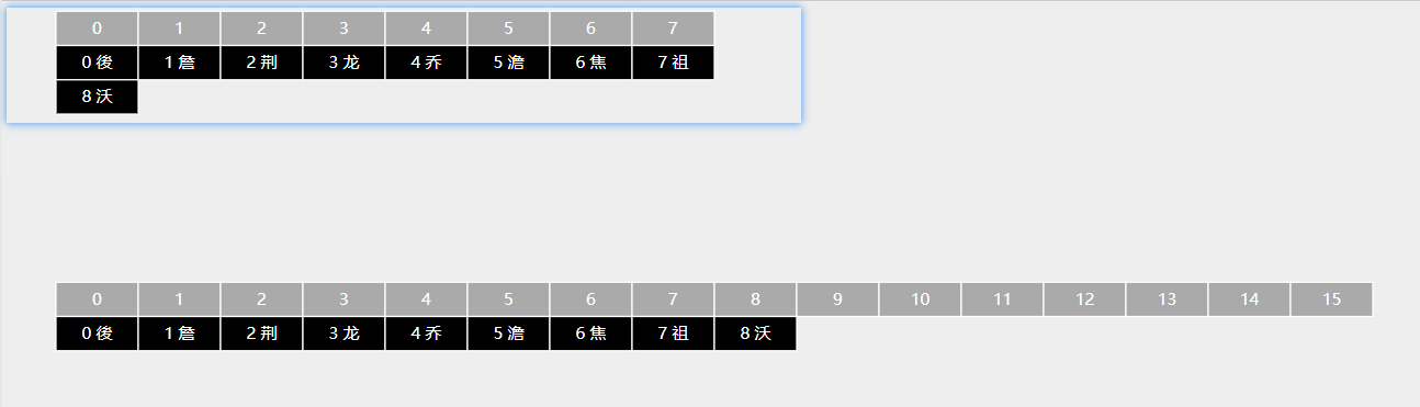
这个拆分是有规律的，前提是数组的长度是2的n次方

• 一个链表最多拆成两个
• hash & table.length == 0 的一组，索引不变
• hash & table.length != 0 的一组，索引是原索引 + table.length
• table.length指的是旧数组长度

为什么是这样？

从二进制的角度出发，扩容一倍，就是余数要多考虑一位，比如从 8 -> 16

容量为8时，余数是后三位，容量为16时，余数是后四位

余数一样的索引一样，会被分配到同一链表

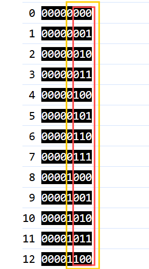
哪些数字扩容后索引不变，哪些数字扩容后索引会变？

很明显，后三位和后四位取值一致的不变，取值不一致的会变，也就是说，多考虑的那一位是0的不变，是1的会变

如何检查多考虑的那一位是0还是1呢？多考虑的那一位保留，其他位置清0，等于0的是0，不等于0的是1

我们需要找到一个数字，它的二进制数在多考虑的那一位是1，其他位置都是0，然后与其他数字做按位与运算，即可达到我们想要的效果

因为 x & 1 = x，x & 0 = 0，比如说，上面这个例子，我们要找的数字就是 8（00001000），检查倒数第4位

8（00001000）& 1（00000001）= 0（00000000），8（00001000）& 9（00001001）= 8（00001000）

8（00001000）& 2（00000010）= 0（00000000），8（00001000）& 10（00001010）= 8（00001000）

而 8 刚好就是旧数组的长度，当然这不是巧合，只要数组长度是2的n次方，这个规律会一直有效

旧数组长度 8 二进制 => 1000 检查倒数第4位
旧数组长度 16 二进制 => 10000 检查倒数第5位

hash & 旧数组长度 就是用来检查扩容前后索引位置（余数）会不会变

为什么拆分后的两条链表，一个原索引不变，另一个是原索引+旧数组长度？

还是看上面那个例子，那些多考虑的那一位是0的扩容前后的后三位和后四位取值一致，所以原索引不变，多考虑的那一位是1的取值不一致，区别在多考虑的那一位多了一个1，所以它们要加上这个1，对应到十进制也就是旧数组长度

private void expand() {
    Entry[] newTable = new Entry[table.length << 1];
    for (int i = 0; i < table.length; i++) {
        Entry p = table[i];
        Entry a = null;
        Entry b = null;
        // 规律： a 链表保持索引位置不变，b 链表索引位置+table.length
        while (p != null) {
            if ((p.hash & table.length) == 0) {
                if (a == null) {
                    // 链表保持索引位置不变
                    newTable[i] = p;
                } else {
                    a.next = p;
                }
                a = p; // 分配到a
            } else {
                if (b == null) {
                    // 链表索引位置+table.length
                    newTable[i + table.length] = p;
                } else {
                    b.next = p;
                }
                b = p; // 分配到b
            }
            p = p.next;
        }
        if (a != null) {
            a.next = null;
        }
        if (b != null) {
            b.next = null;
        }
    }
    table = newTable;
    threshold = (int) (table.length * loadFactor);
}

删除

Object remove(int hash, Object key) {
    int idx = hash & (table.length - 1);
    Entry p = table[idx];
    Entry pre = null;
    while (p != null) {
        if (p.key.equals(key)) {
            // 找到了, 删除
            if (pre == null) { // 头节点
                table[idx] = p.next;
            } else { // 非头节点
                pre.next = p.next;
            }
            size --;
            return p.value;
        }
        pre = p;
        p = p.next;
    }
    //找不到对应key
    return null;
}

哈希算法

哈希算法又叫散列算法和摘要算法

hash 算法是将任意对象，分配一个编号的过程，其中编号是一个有限范围内的数字（如 int 范围内）

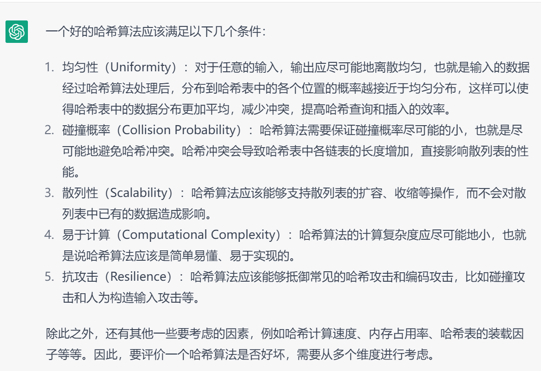
Object.hashCode

• Object 的 hashCode 方法默认是生成随机数作为 hash 值（会缓存在对象头当中），不同的对象生成出来的hashCode不一样
• 缺点是包含相同值的不同对象，他们的 hashCode 不一样，不能够用 hash 值来反映对象的值特征，因此诸多子类都会重写 hashCode 方法

String.hashCode

public static void main(String[] args) {
    String s1 = "bac";                     
    String s2 = new String("abc");         

    System.out.println(s1.hashCode());
    System.out.println(s2.hashCode());

    // 原则：值相同的字符串生成相同的 hash 码, 尽量让值不同的字符串生成不同的 hash 码
    /*
    加权重
    对于 abc  a * 100 + b * 10 + c
    对于 bac  b * 100 + a * 10 + c
     */
    int hash = 0;
    for (int i = 0; i < s1.length(); i++) {
        char c = s1.charAt(i);
        System.out.println((int) c);
        // (a*10 + b)*10 + c  ==>  a*100 + b*10 + c  2^5
        hash = (hash << 5) - hash + c;     
    }
    System.out.println(hash);
}

• 字符串由一个个字符组成，在计算机里每个字符代表一个数字，可以将它们组合起来形成一个hashCode
• 加权重避免 "abc" 和 "bac" 式的哈希冲突（a + b + c = 97 + 98 + 99 = 294，b + a + c = 98 + 97 + 99 = 294）
• 经验表明如果每次乘的是较大质数，可以有更好地降低 hash 冲突，因此改【乘 10】为【乘 31】
• 【乘 31】可以等价为【乘 32 - hash】，进一步可以转为更高效地【左移5位 - hash】

检查 hash 表的分散性

public void print() {
    int[] sum = new int[table.length]; // 存储哈希表中每个链表的长度
    for (int i = 0; i < table.length; i++) {
        Entry p = table[i];
        while (p != null) {
            sum[i]++;
            p = p.next;
        }
    }
    // System.out.println(Arrays.toString(sum));

    Map<Integer, Long> result = Arrays.stream(sum).boxed()
        .collect(Collectors.groupingBy(s -> s, Collectors.counting())); // 分组统计各链表长度的数量
    System.out.println(result);
}

测试

public static void main(String[] args) throws IOException {
    // 测试 Object.hashCode
    HashTable obTable = new HashTable();
    for (int i = 0; i < 200000; i++) {
        Object object = new Object();
        obTable.put(object, object);
    }
    System.out.println("测试 Object.hashCode");
    obTable.print();

    // 测试 String.hashCode
    HashTable strTable = new HashTable();
    List<String> strings = Files.readAllLines(Path.of("words")); // words里有大概20万个字符串
    for (String string : strings) {
        strTable.put(string, string);
    }
    System.out.println("测试 String.hashCode");
    strTable.print();
}

结果

可以看到，效果都不错

其中，都有30多万的格子没有存储元素，造成了空间的浪费，但这个是不可避免的

其他链表长度的数量情况还是挺理想的，链表长度为 1 的占了绝大部分

也没有出现绝大部分数据往少数几个格子里跑的现象，分散性都挺好

MurmurHash

想要在java里使用 MurmurHash，首先要导入谷歌的依赖

<dependency>
    <groupId>com.google.guava</groupId>
    <artifactId>guava</artifactId>
    <version>30.1-jre</version>
</dependency>

它提供了一个 Hashing 工具类，支持很多种不同的 hash 算法，我们使用的是 MurmurHash

int abc = Hashing.murmur3_32().hashString("abc", StandardCharsets.UTF_8).asInt();

其中 3 代表版本，32 代表生成 32 位的 hashCode，hashString 代表针对字符串

检查分散性

可以看到，分散性跟上面两种 hash 算法差不多

最终实现

目前的实现中，我们还需要提供一个参数：hash码，如果是让使用者来提供这个 hash 码，很难保证不发生冲突

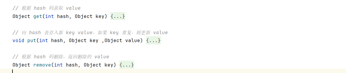
所以我们要改造原来代码，新增一个生成 hash 码的方法和三个对使用者提供的方法

// 获取
Object get(Object key) {
	int hash = hash(key);
    return get(hash, key);
}

// 新增
void put(Object key ,Object value) {
    int hash = hash(key);
    put(hash, key, value);
}

// 删除
Object remove(Object key) {
    int hash = hash(key);
    return remove(hash, key);
}

// 生成 hash 码
private static int hash(Object key) {
    if (key instanceof String k) {
    	return Hashing.murmur3_32().hashString(k, StandardCharsets.UTF_8).asInt();
    }
    return key.hashCode();
}

完整代码

public class HashTable {

    static class Entry {
       int hash; 
       Object key; 
       Object value; 
       Entry next; 

       public Entry(int hash, Object key, Object value) {
           this.hash = hash;
           this.key = key;
           this.value = value;
       }
    }

    Entry[] table = new Entry[16]; 
    int size; 
    float loadFactor = 0.75f; 
    int threshold = (int) (table.length * loadFactor);

    Object get(int hash, Object key) {
        int idx = hash & (table.length - 1);
        Entry p = table[idx];
        while (p != null) {
            if (p.key.equals(key)) {
                return p.value;
            }
            p = p.next;
        }
        return null;
    }

    void put(int hash, Object key ,Object value) {
        int idx = hash & (table.length - 1);
        Entry p = table[idx];
        if (p == null) {
            table[idx] = new Entry(hash, key, value);
        } else {
            while (true) {
                if (p.key.equals(key)) {
                    p.value = value; 
                    return;
                }
                if (p.next == null) {
                    break;
                }
                p = p.next;
            }
            p.next = new Entry(hash, key, value); 
        }
        size++;
        if (size > threshold) { 
            expand();
        }
    }

    Object remove(int hash, Object key) {
        int idx = hash & (table.length - 1);
        Entry p = table[idx];
        Entry pre = null;
        while (p != null) {
            if (p.key.equals(key)) {
                if (pre == null) { 
                    table[idx] = p.next;
                } else { 
                    pre.next = p.next;
                }
                size --;
                return p.value;
            }
            pre = p;
            p = p.next;
        }
        return null;
    }

    private void expand() {
        Entry[] newTable = new Entry[table.length << 1];
        for (int i = 0; i < table.length; i++) {
            Entry p = table[i];
            Entry a = null;
            Entry b = null;
            while (p != null) {
                if ((p.hash & table.length) == 0) {
                    if (a == null) {
                        newTable[i] = p;
                    } else {
                        a.next = p;
                    }
                    a = p; 
                } else {
                    if (b == null) {
                        newTable[i + table.length] = p;
                    } else {
                        b.next = p;
                    }
                    b = p; 
                }
                p = p.next;
            }
            if (a != null) {
                a.next = null;
            }
            if (b != null) {
                b.next = null;
            }
        }
        table = newTable;
        threshold = (int) (table.length * loadFactor);
    }

    Object get(Object key) {
        int hash = hash(key);
        return get(hash, key);
    }

    void put(Object key ,Object value) {
        int hash = hash(key);
        put(hash, key, value);
    }

    Object remove(Object key) {
        int hash = hash(key);
        return remove(hash, key);
    }

    private static int hash(Object key) {
        if (key instanceof String k) {
            return Hashing.murmur3_32().hashString(k, StandardCharsets.UTF_8).asInt();
        }
        return key.hashCode();
    }
}

思考

1. 我们的代码里使用了尾插法，如果改成头插法呢？

   答：没问题，在 Java 中，HashTable用的就是头插法，HashMap在 JDK1.7 及之前用的也是头插法，但其实头插法和尾插法在性能上并没有太大区别，那为什么在 JDK1.8 以后改成了尾插法呢？因为在多线程下，头插法会带来死循环的问题，为了避免这个问题，所以改成了尾插法。

2. JDK 的 HashMap 中采用了将对象 hashCode 高低位相互异或的方式减少冲突，怎么理解？

   答：这样做的目的是混合高位和低位的位信息，避免它们之间的规律性，从而提高哈希值的随机性，减少冲突的概率，优化存储性能。具体实现是：h ^= (h >>> 16)，这将原 hashCode 的高 16 位与低 16 位混合，改善哈希表的分布，提升性能。当然，这样做的前提是 HashMap 的容量是 2 的 n 次方。如果我们使用的不是 2 的 n 次方这种策略，那可以不做异或运算，没什么区别。

3. 我们的 HashTable 中表格容量是 2 的 n 次方，很多优化都是基于这个前提，能否不用 2 的 n 次方作为表格容量？

   答：可以。在 Java 自带的 Hashtable 中，它的初始容量是11，一个质数，它就不是 2 的 n 次方，质数在取模的时候得到的哈希值的分散性会比较好，而 2 的 n 次方它的分散性会比较差，从二进制的角度上看，取模相当于只看了后几位，高位都用不上，所以我们才需要做高低位异或运算。

   但正如题目所说，很多优化都是基于 2 的 n 次方这个前提：

   • 求模 -> 按位与
   • 拆分链表
   • 高低位异或

   如果我们不用 2 的 n 次方作为表格容量，性能会稍逊。

   所以容量是否选择 2 的 n 次方主要是在效率和分散性之间去做选择。

4. JDK 的 HashMap 在链表长度过长会转换成红黑树，对此你怎么看？

   这个操作是在 JDK1.8 后才有的，它会在链表长度超过8的时候将链表转换成红黑树。

   在哈希表中，当多个键值对被映射到同一个位置上（即哈希值相同的情况下），这些键值对会以链表的形式存储。在某些情况下，哈希冲突会导致链表长度过长，这会影响查找、插入、删除等操作的性能。

   但实际上，这个操作主要是为了防患于未然，有的非正常用户会专门造一些相互之间会发生冲突的哈希数据，一旦冲突，就会形成一些非常长的链表，让整个服务器的性能下降，这个时候，这个转换操作可以保底，避免这种恶意攻击对性能造成的影响太大。如果是正常的数据，哈希值分散性比较好，链表长度并不会过长，比如，在前面的例子中，20万的数据量，链表长度最多也只是6，而且也没几个。

图

图是图论的主要研究对象。图是由若干给定的顶点及连接两顶点的边所构成的图形，这种图形通常用来描述某些事物之间的某种特定关系。顶点用于代表事物，连接两顶点的边则用于表示两个事物间具有这种关系。

图论起源于著名的柯尼斯堡七桥问题。该问题于1736年被欧拉解决，因此普遍认为欧拉是图论的创始人。

概念

图是由顶点（vertex）和边（edge）组成的数据结构，例如

该图有四个顶点：A、B、C、D 以及四条有向边，有向图中，边是单向的

有向 VS 无向

如果是无向图，那么边是双向的，下面是一个无向图的例子

度

度是指与该顶点相邻的边的数量

例如上图中

• A、B、C、E、F 这几个顶点度数为 2
• D 顶点度数为 4

有向图中，细分为入度和出度，参见下图

• A (2 out / 0 in)
• B、C、E (1 out / 1 in)
• D (2 out / 2 in)
• F (0 out / 2 in)

权

边可以有权重，代表从源顶点到目标顶点的距离、费用、时间或其他度量。

路径

路径被定义为从一个顶点到另一个顶点的一系列连续边，例如上图中【北京】到【上海】有多条路径

• 北京 - 上海
• 北京 - 武汉 - 上海

路径长度

• 不考虑权重，长度就是边的数量
• 考虑权重，一般就是权重累加

环

在有向图中，从一个顶点开始，可以通过若干条有向边返回到该顶点，那么就形成了一个环

图的连通性

如果两个顶点之间存在路径，则这两个顶点是连通的，所有顶点都连通，则该图被称之为连通图，若子图连通，则称为连通分量

图的表示

比如说，下面的图

用邻接矩阵可以表示为：

  A B C D
A 0 1 1 0
B 1 0 0 1 
C 1 0 0 1
D 0 1 1 0

用邻接表可以表示为：

A -> B -> C
B -> A -> D
C -> A -> D
D -> B -> C

有向图的例子

  A B C D
A 0 1 1 0
B 0 0 0 1
C 0 0 0 1
D 0 0 0 0

A - B - C
B - D
C - D
D - empty

Java 表示

顶点

public class Vertex {
    String name;
    List<Edge> edges;
    
    // 拓扑排序相关
    int inDegree;
    int status; // 状态 0-未访问 1-访问中 2-访问过，用在拓扑排序

    // dfs, bfs 相关
    boolean visited;

    // 求解最短距离相关
    private static final int INF = Integer.MAX_VALUE;
    int dist = INF;
    Vertex prev = null;
}

边

public class Edge {

    Vertex linked;
    int weight;

    public Edge(Vertex linked) {
        this(linked, 1);
    }

    public Edge(Vertex linked, int weight) {
        this.linked = linked;
        this.weight = weight;
    }
}

DFS

public class Dfs {
    public static void main(String[] args) {
        Vertex v1 = new Vertex("v1");
        Vertex v2 = new Vertex("v2");
        Vertex v3 = new Vertex("v3");
        Vertex v4 = new Vertex("v4");
        Vertex v5 = new Vertex("v5");
        Vertex v6 = new Vertex("v6");

        v1.edges = List.of(new Edge(v3), new Edge(v2), new Edge(v6));
        v2.edges = List.of(new Edge(v4));
        v3.edges = List.of(new Edge(v4), new Edge(v6));
        v4.edges = List.of(new Edge(v5));
        v5.edges = List.of();
        v6.edges = List.of(new Edge(v5));

        dfsWithLoop(v1);
    }

    private static void dfsWithLoop(Vertex v) {
        LinkedList<Vertex> stack = new LinkedList<>();
        stack.push(v);
        while (!stack.isEmpty()) {
            Vertex pop = stack.pop();
            pop.visited = true;
            System.out.println(pop.name);
            for (Edge edge : pop.edges) {
                if (!edge.linked.visited) {
                    stack.push(edge.linked);
                }
            }
        }
    }

    private static void dfsWithRecursion(Vertex v) {
        v.visited = true;
        System.out.println(v.name);
        for (Edge edge : v.edges) {
            if (!edge.linked.visited) {
                dfsWithRecursion(edge.linked);
            }
        }
    }
}

BFS

public class Bfs {
    public static void main(String[] args) {
        Vertex v1 = new Vertex("v1");
        Vertex v2 = new Vertex("v2");
        Vertex v3 = new Vertex("v3");
        Vertex v4 = new Vertex("v4");
        Vertex v5 = new Vertex("v5");
        Vertex v6 = new Vertex("v6");

        v1.edges = List.of(new Edge(v3), new Edge(v2), new Edge(v6));
        v2.edges = List.of(new Edge(v4));
        v3.edges = List.of(new Edge(v4), new Edge(v6));
        v4.edges = List.of(new Edge(v5));
        v5.edges = List.of();
        v6.edges = List.of(new Edge(v5));

        bfs(v1);
    }

    private static void bfs(Vertex v) {
        LinkedList<Vertex> queue = new LinkedList<>();
        v.visited = true;
        queue.offer(v);
        while (!queue.isEmpty()) {
            Vertex poll = queue.poll();
            System.out.println(poll.name);
            for (Edge edge : poll.edges) {
                if (!edge.linked.visited) {
                    edge.linked.visited = true;
                    queue.offer(edge.linked);
                }
            }
        }
    }
}

拓补排序

在图论中，拓扑排序（Topological Sorting）是一个有向无环图（DAG, Directed Acyclic Graph）的所有顶点的线性序列。且该序列必须满足下面两个条件：

• 每个顶点出现且只出现一次。
• 若存在一条从顶点 A 到顶点 B 的路径，那么在序列中顶点 A 出现在顶点 B 的前面。

有向无环图（DAG）才有拓扑排序，非DAG图没有拓扑排序一说。

Kahn

基本思想：

• 入度为0的顶点优先：选择当前入度为0的顶点加入结果序列，因为这类顶点不依赖任何其他顶点，符合拓扑排序的要求。
• 动态更新入度：每处理一个顶点，将其邻接顶点的入度减1，模拟“移除”该顶点及其出边。若邻接顶点的入度变为0，则将其加入候选队列。
• 环检测：若最终结果序列的顶点数少于图中总顶点数，说明图中存在环，无法进行拓扑排序。

public class TopologicalSort {
    public static void main(String[] args) {
        Vertex v1 = new Vertex("网页基础");
        Vertex v2 = new Vertex("Java基础");
        Vertex v3 = new Vertex("JavaWeb");
        Vertex v4 = new Vertex("Spring框架");
        Vertex v5 = new Vertex("微服务框架");
        Vertex v6 = new Vertex("数据库");
        Vertex v7 = new Vertex("实战项目");

        v1.edges = List.of(new Edge(v3)); // +1
        v2.edges = List.of(new Edge(v3)); // +1
        v3.edges = List.of(new Edge(v4));
        v6.edges = List.of(new Edge(v4));
        v4.edges = List.of(new Edge(v5));
        v5.edges = List.of(new Edge(v7));
        v7.edges = List.of();

        List<Vertex> graph = List.of(v1, v2, v3, v4, v5, v6, v7);
        // 1. 统计每个顶点的入度
        for (Vertex v : graph) {
            for (Edge edge : v.edges) {
                edge.linked.inDegree++;
            }
        }
        /*for (Vertex vertex : graph) {
            System.out.println(vertex.name + " " + vertex.inDegree);
        }*/
        // 2. 将入度为0的顶点加入队列
        LinkedList<Vertex> queue = new LinkedList<>();
        for (Vertex v : graph) {
            if (v.inDegree == 0) {
                queue.offer(v);
            }
        }
        // 3. 队列中不断移除顶点，每移除一个顶点，把它相邻顶点入度减1，若减到0则入队
        List<String> result = new ArrayList<>();
        while (!queue.isEmpty()) {
            Vertex poll = queue.poll();
//            System.out.println(poll.name);
            result.add(poll.name);
            for (Edge edge : poll.edges) {
                edge.linked.inDegree--;
                if (edge.linked.inDegree == 0) {
                    queue.offer(edge.linked);
                }
            }
        }
        if (result.size() != graph.size()) {
            System.out.println("出现环");
        } else {
            for (String key : result) {
                System.out.println(key);
            }
        }
    }
}

DFS

基本思想：

• 深度优先搜索（DFS）：从任意未访问节点开始，递归访问其邻接节点。
• 标记节点状态：节点有三种状态：
  • 未访问：尚未处理。
  • 访问中：正在递归访问其邻接节点。
  • 已访问：该节点及其邻接节点已处理完毕。
• 完成时间记录：当节点及其邻接节点处理完毕时，将其加入结果列表。
• 结果反转：最终将结果列表反转，得到拓扑排序。

public class TopologicalSortDFS {

    public static void main(String[] args) {
        Vertex v1 = new Vertex("网页基础");
        Vertex v2 = new Vertex("Java基础");
        Vertex v3 = new Vertex("JavaWeb");
        Vertex v4 = new Vertex("Spring框架");
        Vertex v5 = new Vertex("微服务框架");
        Vertex v6 = new Vertex("数据库");
        Vertex v7 = new Vertex("实战项目");

        v1.edges = List.of(new Edge(v3));
        v2.edges = List.of(new Edge(v3));
        v3.edges = List.of(new Edge(v4));
        v6.edges = List.of(new Edge(v4));
        v4.edges = List.of(new Edge(v5));
        v5.edges = List.of(new Edge(v7));
        v7.edges = List.of();

        List<Vertex> graph = List.of(v1, v2, v3, v4, v5, v6, v7);
        LinkedList<String> result = new LinkedList<>();
        for (Vertex v : graph) {
            if(v.status==0) {
                dfs(v, result);
            }
        }
        System.out.println(result);
    }

    private static void dfs(Vertex v, LinkedList<String> result) {
        if (v.status == 2) {
            return;
        }
        if (v.status == 1) {
            throw new RuntimeException("发现环");
        }
        v.status = 1;
        for (Edge edge : v.edges) {
            dfs(edge.linked, result);
        }
        v.status = 2;
        result.push(v.name);
    }
}

最短路径

寻找从某个节点到图中各个节点的最短距离

Dijkstra

算法描述：

1. 将所有顶点标记为未访问。创建一个未访问顶点的集合。
2. 为每个顶点分配一个临时距离值
   • 对于我们的初始顶点，将其设置为零
   • 对于所有其他顶点，将其设置为无穷大。
3. 每次选择最小临时距离的未访问顶点，作为新的当前顶点
4. 对于当前顶点，遍历其所有未访问的邻居，并更新它们的临时距离为更小
   • 例如，1->6 的距离是 14，而1->3->6 的距离是11。这时将距离更新为 11
   • 否则，将保留上次距离值
5. 当前顶点的邻居处理完成后，把它从未访问集合中删除

public class Dijkstra {
    public static void main(String[] args) {
        Vertex v1 = new Vertex("v1");
        Vertex v2 = new Vertex("v2");
        Vertex v3 = new Vertex("v3");
        Vertex v4 = new Vertex("v4");
        Vertex v5 = new Vertex("v5");
        Vertex v6 = new Vertex("v6");

        v1.edges = List.of(new Edge(v3, 9), new Edge(v2, 7), new Edge(v6, 14));
        v2.edges = List.of(new Edge(v4, 15));
        v3.edges = List.of(new Edge(v4, 11), new Edge(v6, 2));
        v4.edges = List.of(new Edge(v5, 6));
        v5.edges = List.of();
        v6.edges = List.of(new Edge(v5, 9));

        List<Vertex> graph = List.of(v1, v2, v3, v4, v5, v6);

        dijkstra(graph, v1);
    }

    private static void dijkstra(List<Vertex> graph, Vertex source) {
        ArrayList<Vertex> list = new ArrayList<>(graph);
        source.dist = 0;

        while (!list.isEmpty()) {
            // 3. 选取当前顶点
            Vertex curr = chooseMinDistVertex(list);
            // 4. 更新当前顶点邻居距离
            updateNeighboursDist(curr, list);
            // 5. 移除当前顶点
            list.remove(curr);
        }

        for (Vertex v : graph) {
            System.out.println(v.name + " " + v.dist);
        }
    }

    private static void updateNeighboursDist(Vertex curr, ArrayList<Vertex> list) {
        for (Edge edge : curr.edges) {
            Vertex n = edge.linked;
            if (list.contains(n)) {
                int dist = curr.dist + edge.weight;
                if (dist < n.dist) {
                    n.dist = dist;
                }
            }
        }
    }

    private static Vertex chooseMinDistVertex(ArrayList<Vertex> list) {
        Vertex min = list.get(0);
        for (int i = 1; i < list.size(); i++) {
            if (list.get(i).dist < min.dist) {
                min = list.get(i);
            }
        }
        return min;
    }

}

改进 - 优先级队列

1. 创建一个优先级队列，放入所有顶点（队列大小会达到边的数量）
2. 为每个顶点分配一个临时距离值
   • 对于我们的初始顶点，将其设置为零
   • 对于所有其他顶点，将其设置为无穷大。
3. 每次选择最小临时距离的未访问顶点，作为新的当前顶点
4. 对于当前顶点，遍历其所有未访问的邻居，并更新它们的临时距离为更小，若距离更新需加入队列
   • 例如，1->6 的距离是 14，而1->3->6 的距离是11。这时将距离更新为 11
   • 否则，将保留上次距离值
5. 当前顶点的邻居处理完成后，把它从队列中删除

public class DijkstraPriorityQueue {
    public static void main(String[] args) {
        Vertex v1 = new Vertex("v1");
        Vertex v2 = new Vertex("v2");
        Vertex v3 = new Vertex("v3");
        Vertex v4 = new Vertex("v4");
        Vertex v5 = new Vertex("v5");
        Vertex v6 = new Vertex("v6");

        v1.edges = List.of(new Edge(v3, 9), new Edge(v2, 7), new Edge(v6, 14));
        v2.edges = List.of(new Edge(v4, 15));
        v3.edges = List.of(new Edge(v4, 11), new Edge(v6, 2));
        v4.edges = List.of(new Edge(v5, 6));
        v5.edges = List.of();
        v6.edges = List.of(new Edge(v5, 9));

        List<Vertex> graph = List.of(v1, v2, v3, v4, v5, v6);

        dijkstra(graph, v1);
    }

    private static void dijkstra(List<Vertex> graph, Vertex source) {
        PriorityQueue<Vertex> queue = new PriorityQueue<>(Comparator.comparingInt(v -> v.dist));
        source.dist = 0;
        for (Vertex v : graph) {
            queue.offer(v);
        }

        while (!queue.isEmpty()) {
            System.out.println(queue);
            // 3. 选取当前顶点
            Vertex curr = queue.peek();
            // 4. 更新当前顶点邻居距离
            if(!curr.visited) {
                updateNeighboursDist(curr, queue);
                curr.visited = true;
            }
            // 5. 移除当前顶点
            queue.poll();
        }

        for (Vertex v : graph) {
            System.out.println(v.name + " " + v.dist + " " + (v.prev != null ? v.prev.name : "null"));
        }
    }

    private static void updateNeighboursDist(Vertex curr, PriorityQueue<Vertex> queue) {
        for (Edge edge : curr.edges) {
            Vertex n = edge.linked;
            if (!n.visited) {
                int dist = curr.dist + edge.weight;
                if (dist < n.dist) {
                    n.dist = dist;
                    n.prev = curr;
                    queue.offer(n);
                }
            }
        }
    }

}

问题

按照 Dijkstra 算法，得出

• v1 -> v2 最短距离2
• v1 -> v3 最短距离1
• v1 -> v4 最短距离2

事实应当是

• v1 -> v2 最短距离2
• v1 -> v3 最短距离0
• v1 -> v4 最短距离1

Bellman-Ford

核心思想：

• 初始化初始顶点的距离为0，其他顶点的距离为无穷大（∞）。
• 对所有的边进行 V - 1 次松弛操作，其中 V 是图中节点的数量。每次松弛操作都会检查每条边，更新目标节点的最短路径估计值。
• 在完成 V - 1 次松弛操作后，检查是否还有边的松弛操作能够更新距离值。如果可以更新，说明图中存在负权环。

为什么是 V - 1 次？

在一个没有负权环的图中，任意两个顶点之间的最短路径最多包含 V - 1 条边。

public class BellmanFord {
    public static void main(String[] args) {
        // 正常情况
        /*Vertex v1 = new Vertex("v1");
        Vertex v2 = new Vertex("v2");
        Vertex v3 = new Vertex("v3");
        Vertex v4 = new Vertex("v4");
        Vertex v5 = new Vertex("v5");
        Vertex v6 = new Vertex("v6");

        v1.edges = List.of(new Edge(v3, 9), new Edge(v2, 7), new Edge(v6, 14));
        v2.edges = List.of(new Edge(v4, 15));
        v3.edges = List.of(new Edge(v4, 11), new Edge(v6, 2));
        v4.edges = List.of(new Edge(v5, 6));
        v5.edges = List.of();
        v6.edges = List.of(new Edge(v5, 9));

        List<Vertex> graph = List.of(v4, v5, v6, v1, v2, v3);*/

        // 负边情况
        /*Vertex v1 = new Vertex("v1");
        Vertex v2 = new Vertex("v2");
        Vertex v3 = new Vertex("v3");
        Vertex v4 = new Vertex("v4");

        v1.edges = List.of(new Edge(v2, 2), new Edge(v3, 1));
        v2.edges = List.of(new Edge(v3, -2));
        v3.edges = List.of(new Edge(v4, 1));
        v4.edges = List.of();
        List<Vertex> graph = List.of(v1, v2, v3, v4);*/

        // 负环情况
        Vertex v1 = new Vertex("v1");
        Vertex v2 = new Vertex("v2");
        Vertex v3 = new Vertex("v3");
        Vertex v4 = new Vertex("v4");

        v1.edges = List.of(new Edge(v2, 2));
        v2.edges = List.of(new Edge(v3, -4));
        v3.edges = List.of(new Edge(v4, 1), new Edge(v1, 1));
        v4.edges = List.of();
        List<Vertex> graph = List.of(v1, v2, v3, v4);

        bellmanFord(graph, v1);
    }

    private static void bellmanFord(List<Vertex> graph, Vertex source) {
        source.dist = 0;
        int size = graph.size();
        // 1. 进行 顶点个数 - 1 轮处理
        for (int i = 0; i < size - 1; i++) {
            // 2. 遍历所有的边
            for (Vertex s : graph) {
                for (Edge edge : s.edges) {
                    // 3. 处理每一条边
                    Vertex e = edge.linked;
                    if (s.dist != Integer.MAX_VALUE && s.dist + edge.weight < e.dist) {
                        e.dist = s.dist + edge.weight;
                        e.prev = s;
                    }
                }
            }
        }
        
        // 负环检测
        for (Vertex s : graph) {
            for (Edge edge : s.edges) {
                Vertex e = edge.linked;
                if (s.dist + edge.weight < e.dist) {
                    throw new RuntimeException("出现负环");
                }
            }
        }
        
        for (Vertex v : graph) {
            System.out.println(v + " " + (v.prev != null ? v.prev.name : "null"));
        }
    }
}

负环

负环指的是环内路径的权重总和是负数，如下图，2 + -4 + 1 = -1，即出现了负环

如果出现负环，环的起点在每一轮绕环结束后起点的最短路径都会被减少，找不到最短路径

在代码中，可以通过这个方法发现负环，如果在【顶点-1】轮处理完成后，还能继续找到更短距离，表示发现了负环

Floyd-Warshall

核心思想：

• 初始化一个距离矩阵 dist[i][j]，矩阵中每个位置表示从节点 i 到节点 j 的临时最短路径。
• 通过三重循环，逐个遍历中介节点 k 更新所有节点对 (i, j) 的最短路径：dist[i][j] = min(dist[i][j], dist[i][k] + dist[k][j])，其实就是逐个判断 i -> k -> j 和 i -> j 哪个是最短路径

public class FloydWarshall {
    public static void main(String[] args) {
        Vertex v1 = new Vertex("v1");
        Vertex v2 = new Vertex("v2");
        Vertex v3 = new Vertex("v3");
        Vertex v4 = new Vertex("v4");

        v1.edges = List.of(new Edge(v3, -2));
        v2.edges = List.of(new Edge(v1, 4), new Edge(v3, 3));
        v3.edges = List.of(new Edge(v4, 2));
        v4.edges = List.of(new Edge(v2, -1));
        List<Vertex> graph = List.of(v1, v2, v3, v4);

        /*
                直接连通
                v1  v2  v3  v4
            v1  0   ∞   -2  ∞
            v2  4   0   3   ∞
            v3  ∞   ∞   0   2
            v4  ∞   -1  ∞   0

                k=0 借助v1到达其它顶点
                v1  v2  v3  v4
            v1  0   ∞   -2  ∞
            v2  4   0   2   ∞
            v3  ∞   ∞   0   2
            v4  ∞   -1  ∞   0

                k=1 借助v2到达其它顶点
                v1  v2  v3  v4
            v1  0   ∞   -2  ∞
            v2  4   0   2   ∞
            v3  ∞   ∞   0   2
            v4  3   -1  1   0

                k=2 借助v3到达其它顶点
                v1  v2  v3  v4
            v1  0   ∞   -2  0
            v2  4   0   2   4
            v3  ∞   ∞   0   2
            v4  3   -1  1   0

                k=3 借助v4到达其它顶点
                v1  v2  v3  v4
            v1  0   -1   -2  0
            v2  4   0   2   4
            v3  5   1   0   2
            v4  3   -1  1   0
         */
        floydWarshall(graph);
    }

    static void floydWarshall(List<Vertex> graph) {
        int size = graph.size();
        int[][] dist = new int[size][size];
        Vertex[][] prev = new Vertex[size][size];
        // 1）初始化
        for (int i = 0; i < size; i++) {
            Vertex v = graph.get(i); // v1 (v3)
            Map<Vertex, Integer> map = v.edges.stream().collect(Collectors.toMap(e -> e.linked, e -> e.weight));
            for (int j = 0; j < size; j++) {
                Vertex u = graph.get(j); // v3
                if (v == u) {
                    dist[i][j] = 0;
                } else {
                    dist[i][j] = map.getOrDefault(u, Integer.MAX_VALUE);
                    prev[i][j] = map.get(u) != null ? v : null;
                }
            }
        }
        print(prev);
        // 2）看能否借路到达其它顶点
        /*
            v2->v1          v1->v?
            dist[1][0]   +   dist[0][0]
            dist[1][0]   +   dist[0][1]
            dist[1][0]   +   dist[0][2]
            dist[1][0]   +   dist[0][3]
         */
        for (int k = 0; k < size; k++) {
            for (int i = 0; i < size; i++) {
                for (int j = 0; j < size; j++) {
//                    dist[i][k]   +   dist[k][j] // i行的顶点，借助k顶点，到达j列顶点
//                    dist[i][j]                  // i行顶点，直接到达j列顶点
                    if (dist[i][k] != Integer.MAX_VALUE &&
                            dist[k][j] != Integer.MAX_VALUE &&
                            dist[i][k] + dist[k][j] < dist[i][j]) {
                        dist[i][j] = dist[i][k] + dist[k][j];
                        prev[i][j] = prev[k][j];
                    }
                }
            }
//            print(dist);
        }
        print(prev);
    }

    static void path(Vertex[][] prev, List<Vertex> graph, int i, int j) {
        LinkedList<String> stack = new LinkedList<>();
        System.out.print("[" + graph.get(i).name + "," + graph.get(j).name + "] ");
        stack.push(graph.get(j).name);
        while (i != j) {
            Vertex p = prev[i][j];
            stack.push(p.name);
            j = graph.indexOf(p);
        }
        System.out.println(stack);
    }

    static void print(int[][] dist) {
        System.out.println("-------------");
        for (int[] row : dist) {
            System.out.println(Arrays.stream(row).boxed()
                    .map(x -> x == Integer.MAX_VALUE ? "∞" : String.valueOf(x))
                    .map(s -> String.format("%2s", s))
                    .collect(Collectors.joining(",", "[", "]")));
        }
    }

    static void print(Vertex[][] prev) {
        System.out.println("-------------------------");
        for (Vertex[] row : prev) {
            System.out.println(Arrays.stream(row).map(v -> v == null ? "null" : v.name)
                    .map(s -> String.format("%5s", s))
                    .collect(Collectors.joining(",", "[", "]")));
        }
    }

}

负环

如果在 3 层循环结束后，在 dist 数组的对角线处（i==j 处）发现了负数，表示出现了负环

最小生成树

有n个节点，寻找能把所有节点连通并且总权重加起来最少的边的集合

Prim

核心思想跟最短路径的Dijkstra算法一致，只是这里按照题目要求我们只看路径的权重就行

public class Prim {
    public static void main(String[] args) {
        Vertex v1 = new Vertex("v1");
        Vertex v2 = new Vertex("v2");
        Vertex v3 = new Vertex("v3");
        Vertex v4 = new Vertex("v4");
        Vertex v5 = new Vertex("v5");
        Vertex v6 = new Vertex("v6");
        Vertex v7 = new Vertex("v7");

        v1.edges = List.of(new Edge(v2, 2), new Edge(v3, 4), new Edge(v4, 1));
        v2.edges = List.of(new Edge(v1, 2), new Edge(v4, 3), new Edge(v5, 10));
        v3.edges = List.of(new Edge(v1, 4), new Edge(v4, 2), new Edge(v6, 5));
        v4.edges = List.of(new Edge(v1, 1), new Edge(v2, 3), new Edge(v3, 2),
                new Edge(v5, 7), new Edge(v6, 8), new Edge(v7, 4));
        v5.edges = List.of(new Edge(v2, 10), new Edge(v4, 7), new Edge(v7, 6));
        v6.edges = List.of(new Edge(v3, 5), new Edge(v4, 8), new Edge(v7, 1));
        v7.edges = List.of(new Edge(v4, 4), new Edge(v5, 6), new Edge(v6, 1));

        List<Vertex> graph = List.of(v1, v2, v3, v4, v5, v6, v7);

        prim(graph, v1);

    }

    static void prim(List<Vertex> graph, Vertex source) {
        ArrayList<Vertex> list = new ArrayList<>(graph);
        source.dist = 0;

        while (!list.isEmpty()) {
            Vertex min = chooseMinDistVertex(list);
            updateNeighboursDist(min);
            list.remove(min);
            min.visited = true;
            System.out.println("---------------");
            for (Vertex v : graph) {
                System.out.println(v);
            }
        }


    }

    private static void updateNeighboursDist(Vertex curr) {
        for (Edge edge : curr.edges) {
            Vertex n = edge.linked;
            if (!n.visited) {
                int dist = edge.weight;
                if (dist < n.dist) {
                    n.dist = dist;
                    n.prev = curr;
                }
            }
        }
    }

    private static Vertex chooseMinDistVertex(ArrayList<Vertex> list) {
        Vertex min = list.get(0);
        for (int i = 1; i < list.size(); i++) {
            if (list.get(i).dist < min.dist) {
                min = list.get(i);
            }
        }
        return min;
    }
}

Kruskal

核心思想：

• 初始化：将所有边按权重从小到大排序。
• 选择边：依次选择权重最小的边，如果这条边的两个顶点不在同一个连通分量中，则将其加入生成树。
• 重复：重复步骤2，直到生成树包含所有顶点，其实我们只要找到 V - 1条边，就代表生成树包含所有顶点，V指顶点数量。

public class Kruskal {
    static class Edge implements Comparable<Edge> {
        List<Vertex> vertices;
        int start;
        int end;
        int weight;

        public Edge(List<Vertex> vertices, int start, int end, int weight) {
            this.vertices = vertices;
            this.start = start;
            this.end = end;
            this.weight = weight;
        }

        public Edge(int start, int end, int weight) {
            this.start = start;
            this.end = end;
            this.weight = weight;
        }

        @Override
        public int compareTo(Edge o) {
            return Integer.compare(this.weight, o.weight);
        }

        @Override
        public String toString() {
            return vertices.get(start).name + "<->" + vertices.get(end).name + "(" + weight + ")";
        }
    }

    public static void main(String[] args) {
        Vertex v1 = new Vertex("v1");
        Vertex v2 = new Vertex("v2");
        Vertex v3 = new Vertex("v3");
        Vertex v4 = new Vertex("v4");
        Vertex v5 = new Vertex("v5");
        Vertex v6 = new Vertex("v6");
        Vertex v7 = new Vertex("v7");

        List<Vertex> vertices = List.of(v1, v2, v3, v4, v5, v6, v7);
        PriorityQueue<Edge> queue = new PriorityQueue<>(List.of(
                new Edge(vertices,0, 1, 2),
                new Edge(vertices,0, 2, 4),
                new Edge(vertices,0, 3, 1),
                new Edge(vertices,1, 3, 3),
                new Edge(vertices,1, 4, 10),
                new Edge(vertices,2, 3, 2),
                new Edge(vertices,2, 5, 5),
                new Edge(vertices,3, 4, 7),
                new Edge(vertices,3, 5, 8),
                new Edge(vertices,3, 6, 4),
                new Edge(vertices,4, 6, 6),
                new Edge(vertices,5, 6, 1)
        ));

        kruskal(vertices.size(), queue);
    }

    static void kruskal(int size, PriorityQueue<Edge> queue) {
        List<Edge> result = new ArrayList<>();
        DisjointSet set = new DisjointSet(size);
        while (result.size() < size - 1) {
            Edge poll = queue.poll();
            int s = set.find(poll.start);
            int e = set.find(poll.end);
            if (s != e) {
                result.add(poll);
                set.union(s, e);
            }
        }

        for (Edge edge : result) {
            System.out.println(edge);
        }
    }
}

不相交集合（并查集合）

验证两个节点之间是否连通

基础

核心思想详解：

【算法与数据结构】—— 并查集-CSDN博客

public class DisjointSet {
    int[] s;
    // 索引对应顶点
    // 元素是用来表示与之有关系的顶点
    /*
        索引  0  1  2  3  4  5  6
        元素 [0, 1, 2, 3, 4, 5, 6] 表示一开始顶点直接没有联系（只与自己有联系）

    */

    public DisjointSet(int size) {
        s = new int[size];
        for (int i = 0; i < size; i++) {
            s[i] = i;
        }
    }

    // find 是找到老大
    public int find(int x) {
        if (x == s[x]) {
            return x;
        }
        return find(s[x]);
    }

    // union 是让两个集合“相交”，即选出新老大，x、y 是原老大索引
    public void union(int x, int y) {
        s[y] = x;
    }

    @Override
    public String toString() {
        return Arrays.toString(s);
    }

}

路径压缩

public int find(int x) { // x = 2
    if (x == s[x]) {
        return x;
    }
    return s[x] = find(s[x]); // 0    s[2]=0
}

Union By Size

public class DisjointSetUnionBySize {
    int[] s;
    int[] size;
    public DisjointSetUnionBySize(int size) {
        s = new int[size];
        this.size = new int[size];
        for (int i = 0; i < size; i++) {
            s[i] = i;
            this.size[i] = 1;
        }
    }

    // find 是找到老大 - 优化：路径压缩
    public int find(int x) { // x = 2
        if (x == s[x]) {
            return x;
        }
        return s[x] = find(s[x]); // 0    s[2]=0
    }

    // union 是让两个集合“相交”，即选出新老大，x、y 是原老大索引
    public void union(int x, int y) {
//        s[y] = x;
        if (size[x] < size[y]) {
            int t = x;
            x = y;
            y = t;
        }
        s[y] = x;
        size[x] = size[x] + size[y];
    }

    @Override
    public String toString() {
        return "内容："+Arrays.toString(s) + "\n大小：" + Arrays.toString(size);
    }
}